Using MachineShop
Melanoma Example
Use of the MachineShop package is demonstrated with a survival analysis example in which the response variable is a censored time to event outcome. Since survival outcomes are a combination of numerical (time to event) and categorical (event) variables, package features for both variable types are illustrated with the example. Support for outcomes other than survival, including nominal and ordinal factors as well as numeric vectors and matrices, is also discussed.
Survival analysis is performed with the Melanoma dataset
from the MASS package (Andersen
et al. 1993). This dataset provides survival time, in days, from
disease treatment to (1) death from disease, (2) alive at study
termination, or (3) death from other causes for 205 Denmark patients
with malignant melanomas. Also provided are potential predictors of the
survival outcomes. The analysis begins by loading required packages
MachineShop, survival (Therneau 2020), and MASS. For
the analysis, a binary overall survival outcome is created by combining
the two death categories (1 and 3) into one.
## Analysis libraries and dataset
library(MachineShop)
library(survival)
data(Melanoma, package = "MASS")

## Malignant melanoma analysis dataset
surv_df <- within(Melanoma, {
  y <- Surv(time, status != 2)
  remove(time, status)
})
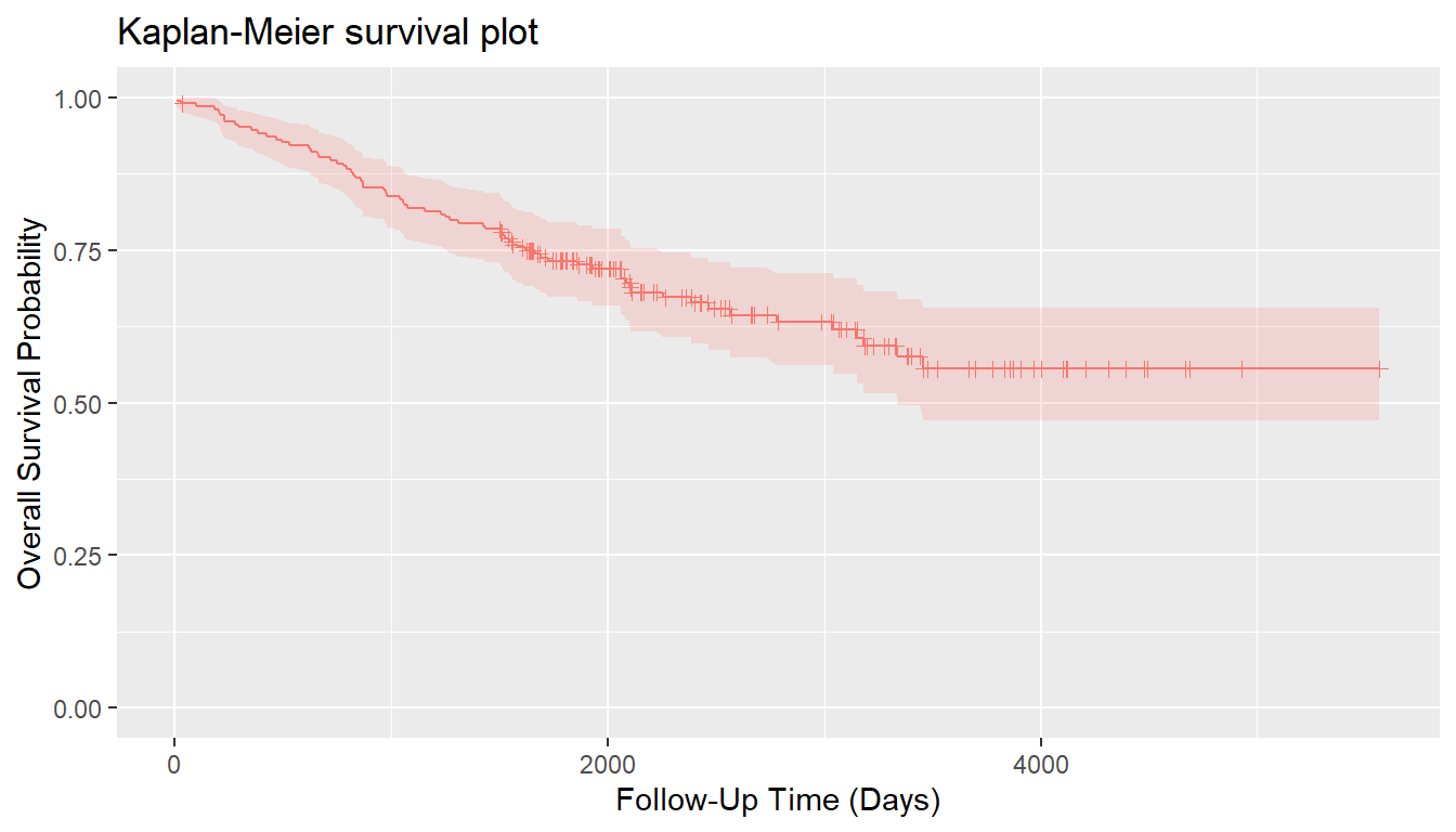
Descriptive summaries of the study variables are given below in Table 1, followed by a plot of estimated overall survival probabilities and 95% confidence intervals.
| Characteristic | Value |
|---|---|
| Number of subjects | 205 |
| time | |
| Median (Range) | 2005 (10, 5565) |
| status | |
| 1 = Dead | 71 (34.63%) |
| 0 = Alive | 134 (65.37%) |
| sex | |
| 1 = Male | 79 (38.54%) |
| 0 = Female | 126 (61.46%) |
| age | |
| Median (Range) | 54 (4, 95) |
| year | |
| Median (Range) | 1970 (1962, 1977) |
| thickness | |
| Median (Range) | 1.94 (0.10, 17.42) |
| ulcer | |
| 1 = Presence | 90 (43.9%) |
| 0 = Absence | 115 (56.1%) |
For the analyses, the dataset is split into a training set on which
survival models will be fit and a test set on which predictions will be
made and performance evaluated. A global formula surv_fo is
defined to relate the predictors on the right hand side to the overall
survival outcome on the left and will be used for all subsequent
survival models.
## Training and test sets
set.seed(123)
train_indices <- sample(nrow(surv_df), nrow(surv_df) * 2 / 3)
surv_train <- surv_df[train_indices, ]
surv_test <- surv_df[-train_indices, ]

## Global formula for the analysis
surv_fo <- y ~ sex + age + year + thickness + ulcer
Model Fit and Prediction
Model Information
Model fitting requires user specification of a
MachineShop compatible model. A named list of
package-supplied models can be obtained interactively with the modelinfo()
function, and includes the following components for each.
label- character descriptor for the model.
packages-
character vector of source packages required to use the model. These
need only be installed with the
install.packages()function or by equivalent means; but need not be loaded with, for example, thelibrary()function. response_types- character vector of response variable types supported by the model.
weights-
logical value or vector of the same length as
response_typesindicating whether case weights are supported for the responses. na.rm-
character sting specifying removal of
"all"cases with missing values from model fitting,"none", or only those whose missing values are in the"response"variable. arguments- closure with the argument names and corresponding default values of the model function.
grid- logical indicating whether automatic generation of tuning parameter grids is implemented for the model.
varimp- logical indicating whether model-specific variable importance is defined.
Function modelinfo()
may be called without arguments, with one or more model functions,
observed response variables, or vectors representing response variable
types; and will return information on all matching models.
## All available models
modelinfo() %>% names
#>  [1] "AdaBagModel"         "AdaBoostModel"       "BARTMachineModel"
#>  [4] "BARTModel"           "BlackBoostModel"     "C50Model"
#>  [7] "CForestModel"        "CoxModel"            "CoxStepAICModel"
#> [10] "EarthModel"          "FDAModel"            "GAMBoostModel"
#> [13] "GBMModel"            "GLMBoostModel"       "GLMModel"
#> [16] "GLMStepAICModel"     "GLMNetModel"         "KNNModel"
#> [19] "LARSModel"           "LDAModel"            "LMModel"
#> [22] "MDAModel"            "NaiveBayesModel"     "NNetModel"
#> [25] "ParsnipModel"        "PDAModel"            "PLSModel"
#> [28] "POLRModel"           "QDAModel"            "RandomForestModel"
#> [31] "RangerModel"         "RFSRCModel"          "RPartModel"
#> [34] "SelectedModel"       "StackedModel"        "SuperModel"
#> [37] "SurvRegModel"        "SurvRegStepAICModel" "SVMModel"
#> [40] "SVMANOVAModel"       "SVMBesselModel"      "SVMLaplaceModel"
#> [43] "SVMLinearModel"      "SVMPolyModel"        "SVMRadialModel"
#> [46] "SVMSplineModel"      "SVMTanhModel"        "TreeModel"
#> [49] "TunedModel"          "XGBModel"            "XGBDARTModel"
#> [52] "XGBLinearModel"      "XGBTreeModel"
Information is displayed below for the GBMModel()
function corresponding to a generalized boosted regression model, which
is applicable to survival outcomes.
## Model-specific information
modelinfo(GBMModel)
#> $GBMModel
#> $GBMModel$label
#> [1] "Generalized Boosted Regression"
#>
#> $GBMModel$packages
#> [1] "gbm"
#>
#> $GBMModel$response_types
#> [1] "factor"         "numeric"        "PoissonVariate" "Surv"
#>
#> $GBMModel$weights
#> [1] TRUE
#>
#> $GBMModel$na.rm
#> [1] "response"
#>
#> $GBMModel$arguments
#> function (distribution = character(), n.trees = 100, interaction.depth = 1,
#>     n.minobsinnode = 10, shrinkage = 0.1, bag.fraction = 0.5)
#> NULL
#>
#> $GBMModel$grid
#> [1] TRUE
#>
#> $GBMModel$varimp
#> [1] TRUE
Submitting the model function at the console will result in similar information being displayed as formatted text.
GBMModel
#> --- MLModelFunction object --------------------------------------------------
#>
#> Model name: GBMModel
#> Label: Generalized Boosted Regression
#> Package: gbm
#> Response types: factor, numeric, PoissonVariate, Surv
#> Case weights support: TRUE
#> Missing case removal: response
#> Tuning grid: TRUE
#> Variable importance: TRUE
#>
#> Arguments:
#> function (distribution = character(), n.trees = 100, interaction.depth = 1,
#>     n.minobsinnode = 10, shrinkage = 0.1, bag.fraction = 0.5)
#> NULL
Type-Specific Models
When data objects are supplied as arguments to modelinfo(),
information is returned on all models applicable to response variables
of the same data types. If model functions are additionally supplied as
arguments, information on the subset matching the data types is
returned.
## All survival response-specific models
modelinfo(Surv(0)) %>% names
#>  [1] "BARTModel"           "BlackBoostModel"     "CForestModel"
#>  [4] "CoxModel"            "CoxStepAICModel"     "GAMBoostModel"
#>  [7] "GBMModel"            "GLMBoostModel"       "GLMNetModel"
#> [10] "ParsnipModel"        "RangerModel"         "RFSRCModel"
#> [13] "RPartModel"          "SelectedModel"       "StackedModel"
#> [16] "SuperModel"          "SurvRegModel"        "SurvRegStepAICModel"
#> [19] "TunedModel"          "XGBModel"            "XGBDARTModel"
#> [22] "XGBLinearModel"      "XGBTreeModel"

## Identify survival response-specific models
modelinfo(Surv(0), CoxModel, GBMModel, SVMModel) %>% names
#> [1] "CoxModel" "GBMModel"
Response Variable-Specific Models
As a special case of type-specific arguments, existing response variables to be used in analyses may be given as arguments to identify applicable models.
## Models for a responses variable
modelinfo(surv_df$y) %>% names
#>  [1] "BARTModel"           "BlackBoostModel"     "CForestModel"
#>  [4] "CoxModel"            "CoxStepAICModel"     "GAMBoostModel"
#>  [7] "GBMModel"            "GLMBoostModel"       "GLMNetModel"
#> [10] "ParsnipModel"        "RangerModel"         "RFSRCModel"
#> [13] "RPartModel"          "SelectedModel"       "StackedModel"
#> [16] "SuperModel"          "SurvRegModel"        "SurvRegStepAICModel"
#> [19] "TunedModel"          "XGBModel"            "XGBDARTModel"
#> [22] "XGBLinearModel"      "XGBTreeModel"
Fit Function
Package models, such as GBMModel,
can be specified in the model argument of the fit()
function to estimate a relationship (surv_fo) between
predictors and an outcome based on a set of data
(surv_train). Argument specifications may be in terms of a
model function, function name, or object.
## Generalized boosted regression fit

## Model function
surv_fit <- fit(surv_fo, data = surv_train, model = GBMModel)

## Model function name
fit(surv_fo, data = surv_train, model = "GBMModel")

## Model object
fit(surv_fo, data = surv_train, model = GBMModel(n.trees = 100, interaction.depth = 1))
Model function arguments will assume their default values unless otherwise changed in a function call.
Dynamic Model Parameters
Dynamic model parameters are model function arguments
defined as expressions to be evaluated at the time of model fitting. As
such, their values can change based on characteristics of the analytic
dataset, including the number of observations or predictor variables.
Expressions to dynamic parameters are specified within the
package-supplied quote operator .()
and can include the following objects:
nobs-
number of observations in
data. nvars-
number of predictor variables in
data. y- response variable.
In the example below, Bayesian information criterion (BIC) based
stepwise variable selection is performed by creating a CoxStepAICModel
with dynamic parameter k to be calculated as the log number
of observations in the fitted dataset.
## Dynamic model parameter k = log number of observations

## Number of observations: nobs
fit(surv_fo, data = surv_train, model = CoxStepAICModel(k = .(log(nobs))))

## Response variable: y
fit(surv_fo, data = surv_train, model = CoxStepAICModel(k = .(log(length(y)))))
Predict Function
A predict()
function is supplied for application to model fit results to obtain
predicted values on a dataset specified with its newdata
argument or on the original dataset if not specified. Survival means are
predicted for survival outcomes by default. Estimates of the associated
survival distributions are needed to calculate the means. For models,
like GBMModel,
that perform semi- or non-parametric survival analysis, Weibull
approximations to the survival distributions are the default for mean
estimation. Other choices of distributional approximations are
exponential, Rayleigh, and empirical. Empirical distributions are
applicable to Cox proportional hazards-based models and can be
calculated with the method of Breslow (1972) or Efron (1977,
default). Note, however, that empirical survival means are
undefined mathematically if an event does not occur at the longest
follow-up time. In such situations, a restricted survival mean is
calculated by changing the longest follow-up time to an event, as
suggested by Efron (1967), which will be
negatively biased.
## Predicted survival means (default: Weibull distribution)
predict(surv_fit, newdata = surv_test)
#> --- SurvMeans object --------------------------------------------------------
#>  [1]   980.6426  8355.2097 19092.0713  1657.1081  2435.7916  7423.9210
#>  [7]   980.6426   765.2302  3002.7963  3544.1334
#> ... with 59 more values
#> Distribution: weibull

## Predicted survival means (empirical distribution)
predict(surv_fit, newdata = surv_test, distr = "empirical")
#> --- SurvMeans object --------------------------------------------------------
#>  [1] 1237.336 4806.528 5275.550 2174.870 2982.527 4699.455 1237.336  936.588
#>  [9] 3399.671 3703.666
#> ... with 59 more values
#> Distribution: empirical
In addition to survival means, predicted survival probabilities
(type = "prob") or 0-1 survival events (default:
type = "response") can be obtained with the follow-up
times argument. The cutoff probability for classification
of survival events (or other binary responses) can be set optionally
with the cutoff argument (default:
cutoff = 0.5). As with mean estimation, distributional
approximations to the survival functions may be specified for the
predictions, with the default for survival probabilities being the
empirical distribution.
## Predict survival probabilities and events at specified follow-up times
surv_times <- 365 * c(5, 10)

predict(surv_fit, newdata = surv_test, times = surv_times, type = "prob")
#> --- SurvProbs object --------------------------------------------------------
#>            Time1      Time2
#>  [1,] 0.17831449 0.05242217
#>  [2,] 0.88497752 0.81143387
#>  [3,] 0.95693579 0.92748997
#>  [4,] 0.40584818 0.21394117
#>  [5,] 0.57104030 0.38361499
#>  [6,] 0.86814014 0.78521296
#>  [7,] 0.17831449 0.05242217
#>  [8,] 0.09609059 0.01821231
#>  [9,] 0.64879179 0.47719578
#> [10,] 0.70290781 0.54725952
#> ... with 59 more rows
#> Times: 1825, 3650
#> Distribution: empirical

predict(surv_fit, newdata = surv_test, times = surv_times, cutoff = 0.7)
#> --- SurvEvents object -------------------------------------------------------
#>       Time1 Time2
#>  [1,]     1     1
#>  [2,]     0     0
#>  [3,]     0     0
#>  [4,]     1     1
#>  [5,]     1     1
#>  [6,]     0     0
#>  [7,]     1     1
#>  [8,]     1     1
#>  [9,]     1     1
#> [10,]     0     1
#> ... with 59 more rows
#> Times: 1825, 3650
#> Distribution: empirical
Prediction of other outcome types is more straightforward. Predicted
numeric and factor responses are of the same class as the observed
values at the default type = "response"; whereas, double
(decimal) numeric values and factor level probabilities result when
type = "prob".
Variable Specifications
Variable specification defines the relationship between response and
predictor variables as well as the data used to estimate the
relationship. Four main types of specifications are supported by the
package’s fit()
and resample()
functions: traditional formula, design matrix, model frame, and
recipe.
Traditional Formula
Variables may be specified with a traditional formula and data frame
pair, as was done at the start of the survival example. This
specification allows for crossing (*), interaction
(:), and removal (-) of predictors in the
formula; . substitution of variables not already appearing
in the formula; in-line functions of response variables; and in-lining
of operators and functions of predictors.
## Datasets
data(Pima.te, package = "MASS")
data(Pima.tr, package = "MASS")

## Formula specification
model_fit <- fit(type ~ ., data = Pima.tr, model = GBMModel)
predict(model_fit, newdata = Pima.te) %>% head
#> [1] Yes No  No  No  No  Yes
#> Levels: No Yes
The syntax for traditional formulas is detailed in the
R help documentation on the formula()
function. However, some constraints are placed on the syntax by the
MachineShop package. Specifically, in-lining on the
right-hand side of formulas is limited to the operators and functions
listed in the "RHS.formula" package setting.
settings("RHS.formula")
#>  [1] "!"        "!="       "%%"       "%/%"      "%in%"     "&"
#>  [7] "("        "*"        "+"        "-"        "."        "/"
#> [13] ":"        "<"        "<="       "=="       ">"        ">="
#> [19] "I"        "^"        "abs"      "acos"     "acosh"    "asin"
#> [25] "asinh"    "atan"     "atanh"    "ceiling"  "cos"      "cosh"
#> [31] "cospi"    "digamma"  "exp"      "expm1"    "floor"    "gamma"
#> [37] "lgamma"   "log"      "log1p"    "offset"   "round"    "sign"
#> [43] "signif"   "sin"      "sinh"     "sinpi"    "sqrt"     "tan"
#> [49] "tanh"     "tanpi"    "trigamma" "trunc"    "|"
This setting is intended to help avoid the definition of predictor
variable encodings that involve dataset-specific parameter calculations.
Such parameters would be calculated separated on training and test sets,
and could lead to failed calculations or improper estimates of
predictive performance. For example, the factor() function
is not allowed because consistency of its (default) encoding requires
that all levels be present in every dataset. Resampled datasets subset
the original cases and are thus prone to missing factor levels. For
users wishing to apply factor encodings or other encodings not available
with traditional formulas, a more flexible preprocessing recipe syntax
is supported, as described later.
Design Matrix
Variables stored separately in a design matrix of predictors and
object of responses can be supplied to the fit functions directly.
Fitting with design matrices has less computational overhead than
traditional formulas and allows for greater numbers of predictor
variables in some models, including GBMModel,
GLMNetModel,
and RandomForestModel.
## Example design matrix and response object
x <- model.matrix(type ~ . - 1, data = Pima.tr)
y <- Pima.tr$type

## Design matrix specification
model_fit <- fit(x, y, model = GBMModel)
predict(model_fit, newdata = Pima.te) %>% head
#> [1] Yes No  No  No  No  Yes
#> Levels: No Yes
Model Frame
A ModelFrame
class is defined by the package for specification of predictor and
response variables along with other attributes to control model fitting.
Model frames can be created with calls to the ModelFrame()
constructor function using a syntax similar to the traditional formula
or design matrix.
## Model frame specification

## Formula
mf <- ModelFrame(type ~ ., data = Pima.tr)
model_fit <- fit(mf, model = GBMModel)
predict(model_fit, newdata = Pima.te) %>% head
#> [1] Yes No  No  No  No  Yes
#> Levels: No Yes

## Design matrix
mf <- ModelFrame(x, y)
model_fit <- fit(mf, model = GBMModel)
predict(model_fit, newdata = Pima.te) %>% head
#> [1] Yes No  No  No  No  Yes
#> Levels: No Yes
The model frame approach has a few advantages over model fitting
directly with a traditional formula. One is that cases with missing
values on any of the response or predictor variables are excluded from
the model frame by default. This is often desirable for models that do
not handle missing values. Conversely, missing values can be retained in
the model frame by setting its argument na.rm = FALSE for
models, like GBMModel,
that do handle them. A second advantage is that case weights can be
included in the model frame to be passed on to the model fitting
functions.
## Model frame specification with case weights
mf <- ModelFrame(ncases / (ncases + ncontrols) ~ agegp + tobgp + alcgp, data = esoph,
                 weights = ncases + ncontrols)
fit(mf, model = GBMModel)
A third, which will be illustrated later, is user-specification of a
variable for stratified resampling via the constructor’s
strata argument.
Preprocessing Recipe
The recipes package (Kuhn and Wickham 2020) provides a flexible framework for defining predictor and response variables as well as preprocessing steps to be applied to them prior to model fitting. Using recipes helps ensure that estimation of predictive performance accounts for all modeling step. They are also a convenient way of consistently applying preprocessing to new data. A basic recipe is given below in terms of the formula and data frame ingredients needed for the analysis.
## Recipe specification
library(recipes)

rec <- recipe(type ~ ., data = Pima.tr)
model_fit <- fit(rec, model = GBMModel)
predict(model_fit, newdata = Pima.te) %>% head
#> [1] Yes No  No  No  Yes Yes
#> Levels: No Yes
As shown, prediction on new data with a model fit to a recipe is done
on an unprocessed dataset. Recipe case weights and stratified resampling
are supported with the role_case()
function. As an example, an initial step is included in the recipe below
to replace the original role of variable weights with a
designation of case weights. That is followed by a step to convert three
ordinal factors to integer scores.
## Recipe specification with case weights
df <- within(esoph, {
  y <- ncases / (ncases + ncontrols)
  weights <- ncases + ncontrols
  remove(ncases, ncontrols)
})

rec <- recipe(y ~ agegp + tobgp + alcgp + weights, data = df) %>%
  role_case(weight = weights, replace = TRUE) %>%
  step_ordinalscore(agegp, tobgp, alcgp)
fit(rec, model = GBMModel)
Summary
The variable specification approaches differ with respect to support for preprocessing, in-line functions, case weights, resampling strata, and computational overhead, as summarized in the table below. Only recipes apply preprocessing steps automatically during model fitting and should be used when it is important to account for such steps in the estimation of model predictive performance. Preprocessing would need to be done manually and separately otherwise. Design matrices have the lowest computational overhead and can enable analyses involving larger numbers of predictors than the other approaches. Both recipes and model frames allow for user-defined case weights (default: equal) and resampling strata (default: none). The remaining approaches are fixed to have equal weights and strata defined by the response variable. Syntax ranges from simplest to most complex for design matrices, traditional formulas, model frames, and recipes, respectively. The relative strengths of each approach should be considered within the context of a given analysis when deciding upon which one to use.
| Specification | Preprocessing | In-line Functions | Case Weights | Resampling Strata | Computational Overhead |
|---|---|---|---|---|---|
| Traditional Formula | manual | yes | equal | response | medium |
| Design Matrix | manual | no | equal | response | low |
| Model Frame | |||||
| Traditional Formula | manual | yes | user | user | medium |
| Design Matrix | manual | no | user | user | low |
| Recipe | automatic | no | user | user | high |
Response Variable Types
The R class types of response variables play a central role in their analysis with the package. They determine, for example, the specific models that can be fit, fitting algorithms employed, predicted values produced, and applicable performance metrics and analyses. As described in the following sections, factors, ordered factors, numeric vectors and matrices, and survival objects are supported by the package.
Factor
Categorical responses with two or more levels should be coded as a
factor variable for analysis. Prediction is of factor
levels by default and of level-specific probabilities if
type = "prob".
## Iris flowers species (3-level factor)
model_fit <- fit(Species ~ ., data = iris, model = GBMModel)
predict(model_fit) %>% head
#> [1] setosa setosa setosa setosa setosa setosa
#> Levels: setosa versicolor virginica
predict(model_fit, type = "prob") %>% head
#>         setosa   versicolor    virginica
#> [1,] 0.9999529 4.704617e-05 5.999170e-08
#> [2,] 0.9999732 2.667703e-05 1.626995e-07
#> [3,] 0.9999744 2.549026e-05 7.312256e-08
#> [4,] 0.9999683 3.164919e-05 1.004487e-07
#> [5,] 0.9999529 4.704617e-05 5.999170e-08
#> [6,] 0.9999446 5.537937e-05 5.999120e-08
In the case of a binary factor, the second factor level is treated as the event and the level for which predicted probabilities are computed.
## Pima Indians diabetes statuses (binary factor)
data(Pima.te, package = "MASS")
data(Pima.tr, package = "MASS")

model_fit <- fit(type ~ ., data = Pima.tr, model = GBMModel)
predict(model_fit, newdata = Pima.te) %>% head
#> [1] Yes No  No  No  No  Yes
#> Levels: No Yes
predict(model_fit, newdata = Pima.te, type = "prob") %>% head
#> [1] 0.84469494 0.05769275 0.03483727 0.03271784 0.48315264 0.74959442
Ordered Factor
Categorical responses can be designated as having ordered levels by
storing them as an ordered factor variable. For categorical
vectors, this can be accomplished with the factor()
function and its argument ordered = TRUE or more simply
with the ordered() function. Numeric vectors can be
converted to ordered factors with the cut() function.
## Iowa City housing prices (ordered factor)
df <- within(ICHomes, {
  sale_amount <- cut(sale_amount, breaks = 3,
                     labels = c("Low", "Medium", "High"),
                     ordered_result = TRUE)
})

model_fit <- fit(sale_amount ~ ., data = df, model = GBMModel)
predict(model_fit) %>% head
#> [1] Low Low Low Low Low Low
#> Levels: Low < Medium < High
predict(model_fit, type = "prob") %>% head
#>            Low      Medium         High
#> [1,] 0.9964837 0.003459652 5.669359e-05
#> [2,] 0.9970031 0.002944093 5.276251e-05
#> [3,] 0.9852936 0.014556622 1.498127e-04
#> [4,] 0.9842968 0.015583572 1.195963e-04
#> [5,] 0.9184646 0.081327684 2.077245e-04
#> [6,] 0.8934669 0.106306241 2.268354e-04
Numeric Vector
Code univariate numerical responses as a numeric
variable. Predicted numeric values are of the original type (integer or
double) by default, and doubles if type = "numeric".
## Iowa City housing prices
model_fit <- fit(sale_amount ~ ., data = ICHomes, model = GBMModel)
predict(model_fit) %>% head
#> [1] 105664 171728 205150 120392 218505 225576
predict(model_fit, type = "numeric") %>% head
#> [1] 105663.7 171727.6 205149.8 120392.4 218504.6 225576.3
Numeric Matrix
Store multivariate numerical responses as a numeric
matrix variable for model fitting with traditional formulas
and model frames.
## Anscombe's multiple regression models dataset

## Numeric matrix response formula
model_fit <- fit(cbind(y1, y2, y3) ~ x1, data = anscombe, model = LMModel)
predict(model_fit) %>% head
#>             y1        y2       y3
#> [1,]  8.001000  8.000909 7.999727
#> [2,]  7.000818  7.000909 7.000273
#> [3,]  9.501273  9.500909 9.498909
#> [4,]  7.500909  7.500909 7.500000
#> [5,]  8.501091  8.500909 8.499455
#> [6,] 10.001364 10.000909 9.998636
For recipes, the multiple response may be defined on the left hand side of a recipe formula or as a single variable within a data frame.
## Numeric matrix response recipe
## Defined in a recipe formula
rec <- recipe(y1 + y2 + y3 ~ x1, data = anscombe)

## Defined within a data frame
df <- within(anscombe, {
  y <- cbind(y1, y2, y3)
  remove(y1, y2, y3)
})
rec <- recipe(y ~ x1, data = df)
model_fit <- fit(rec, model = LMModel)
predict(model_fit) %>% head
#>             y1        y2       y3
#> [1,]  8.001000  8.000909 7.999727
#> [2,]  7.000818  7.000909 7.000273
#> [3,]  9.501273  9.500909 9.498909
#> [4,]  7.500909  7.500909 7.500000
#> [5,]  8.501091  8.500909 8.499455
#> [6,] 10.001364 10.000909 9.998636
Survival Objects
Censored time-to-event survival responses should be stored as a
Surv variable for model fitting with traditional formulas
and model frames.
## Survival response formula
library(survival)

fit(Surv(time, status) ~ ., data = veteran, model = GBMModel)
For recipes, survival responses may be defined with the individual
survival time and event variables given on the left hand side of a
recipe formula and their roles designated with the role_surv()
function or as a single Surv variable within a data
frame.
## Survival response recipe
## Defined in a recipe formula
rec <- recipe(time + status ~ ., data = veteran) %>%
  role_surv(time = time, event = status)

## Defined within a data frame
df <- within(veteran, {
  y <- Surv(time, status)
  remove(time, status)
})
rec <- recipe(y ~ ., data = df)
fit(rec, model = GBMModel)
Model Performance Metrics
Performance metrics quantify associations between observed and predicted responses and provide a means of evaluating the predictive performances of models.
Performance Function
Metrics can be computed with the performance()
function applied to observed responses and responses predicted with the
predict()
function. In the case of observed versus predicted survival
probabilities or events, metrics will be calculated at user-specified
survival times and returned along with their time-integrated mean.
## Survival performance metrics

## Observed responses
obs <- response(surv_fit, newdata = surv_test)

## Predicted survival means
pred_means <- predict(surv_fit, newdata = surv_test)
performance(obs, pred_means)
#>  C-Index
#> 0.622093

## Predicted survival probabilities
pred_probs <- predict(surv_fit, newdata = surv_test, times = surv_times, type = "prob")
performance(obs, pred_probs)
#>     Brier.Mean    Brier.Time1    Brier.Time2   ROC AUC.Mean  ROC AUC.Time1
#>      0.2775278      0.2310083      0.3240473      0.6053896      0.6091172
#>  ROC AUC.Time2  Accuracy.Mean Accuracy.Time1 Accuracy.Time2
#>      0.6016620      0.6667354      0.7207325      0.6127383

## Predicted survival events
pred_events <- predict(surv_fit, newdata = surv_test, times = surv_times)
performance(obs, pred_events)
#>  Accuracy.Mean Accuracy.Time1 Accuracy.Time2
#>      0.6667354      0.7207325      0.6127383
Function performance()
computes a default set of metrics according to the observed and
predicted response types, as indicated and in the order given in the
table below.
Table 3. Default performance metrics by response types.
| Response | Default Metrics |
|---|---|
| Factor | Brier Score, Accuracy, Cohen’s Kappa |
| Binary Factor | Brier Score, Accuracy, Cohen’s Kappa, Area Under ROC Curve, Sensitivity, Specificity |
| Numeric Vector or Matrix | Root Mean Squared Error, R2, Mean Absolute Error |
| Survival Means | Concordance Index |
| Survival Probabilities | Brier Score, Area Under ROC Curve, Accuracy |
| Survival Events | Accuracy |
These defaults may be changed by specifying one or more
package-supplied metric functions to the metrics argument
of performance().
Specification of the metrics argument can be in terms of a
single metric function, function name, or list of metric functions. List
names, if specified, will be displayed as metric labels in graphical and
tabular summaries; otherwise, the function names will be used as labels
for unnamed lists.
## Single metric function
performance(obs, pred_means, metrics = cindex)

## Single metric function name
performance(obs, pred_means, metrics = "cindex")

## List of metric functions
performance(obs, pred_means, metrics = c(cindex, rmse, rmsle))

## Named list of metric functions
performance(obs, pred_means,
            metrics = c("CIndex" = cindex, "RMSE" = rmse, "RMSLE" = rmsle))
Metrics based on classification of two-level class probabilities,
like sensitivity and specificity, optionally allow for specification of
the classification cutoff probability (default:
cutoff = 0.5).
## User-specified survival probability metrics
performance(obs, pred_probs, metrics = c(sensitivity, specificity), cutoff = 0.7)
#>  sensitivity.Mean sensitivity.Time1 sensitivity.Time2  specificity.Mean
#>         0.4855464         0.4636436         0.5074493         0.6655982
#> specificity.Time1 specificity.Time2
#>         0.7487698         0.5824266
Metric Functions
Whereas multiple package-supplied metrics can be calculated
simultaneously with the performance()
function, each exists as a stand-alone function that can be called
individually.
## Metric functions for survival means
cindex(obs, pred_means)
#> [1] 0.622093

rmse(obs, pred_means)
#> [1] 5463.385

rmsle(obs, pred_means)
#> [1] 1.998432

## Metric functions for survival probabilities
sensitivity(obs, pred_probs)
#>      Mean     Time1     Time2
#> 0.3588005 0.2895285 0.4280725

specificity(obs, pred_probs)
#>      Mean     Time1     Time2
#> 0.9323417 0.8646834 1.0000000
Metric Information
A named list of available metrics can be obtained interactively with
the metricinfo()
function, and includes the following components for each one.
label- character descriptor for the metric.
maximize- logical indicating whether maximization of the metric leads to better predictive performance.
arguments- closure with the argument names and corresponding default values of the metric function.
response_types- data frame of the observed and predicted response variable types supported by the metric.
Function metricinfo()
may be called without arguments, with one or more metric functions, an
observed response variable, an observed and predicted response variable
pair, response variable types, or resampled output; and will return
information on all matching metrics.
## All available metrics
metricinfo() %>% names
#>  [1] "accuracy"        "auc"             "brier"           "cindex"
#>  [5] "cross_entropy"   "f_score"         "fnr"             "fpr"
#>  [9] "gini"            "kappa2"          "mae"             "mse"
#> [13] "msle"            "npv"             "ppr"             "ppv"
#> [17] "pr_auc"          "precision"       "r2"              "recall"
#> [21] "rmse"            "rmsle"           "roc_auc"         "roc_index"
#> [25] "sensitivity"     "specificity"     "tnr"             "tpr"
#> [29] "weighted_kappa2"
Information is displayed below for the cindex()
function corresponding to a concordance index, which is applicable to
observed survival and predicted means.
## Metric-specific information
metricinfo(cindex)
#> $cindex
#> $cindex$label
#> [1] "Concordance Index"
#>
#> $cindex$maximize
#> [1] TRUE
#>
#> $cindex$arguments
#> function (observed, predicted = NULL, weights = NULL, ...)
#> NULL
#>
#> $cindex$response_types
#>   observed predicted
#> 1   factor   numeric
#> 2 Resample      NULL
#> 3     Surv   numeric
Submitting the metric function at the console will result in similar information being displayed as formatted text.
cindex
#> --- MLMetric object ---------------------------------------------------------
#>
#> Metric name: cindex
#> Label: Concordance Index
#> Maximize: TRUE
#>
#> Arguments:
#> function (observed, predicted = NULL, weights = NULL, ...)
#> NULL
#>
#> Types:
#>   observed predicted
#> 1   factor   numeric
#> 2 Resample      NULL
#> 3     Surv   numeric
Type-Specific Metrics
When data objects are supplied as arguments to metricinfo(),
information is returned on all metrics applicable to response variables
of the same data types. Observed response variable type is inferred from
the first data argument and predicted type from the second, if given.
For survival responses, predicted types may be numeric for
survival means, SurvEvents
for 0-1 survival events at specified follow-up times, or SurvProbs
for follow-up time survival probabilities. If model functions are
additionally supplied as arguments, information on the subset matching
the data types is returned.
## Metrics for observed and predicted response variable types
metricinfo(Surv(0)) %>% names
#>  [1] "accuracy"    "auc"         "brier"       "cindex"      "f_score"
#>  [6] "fnr"         "fpr"         "gini"        "kappa2"      "mae"
#> [11] "mse"         "msle"        "npv"         "ppr"         "ppv"
#> [16] "pr_auc"      "precision"   "r2"          "recall"      "rmse"
#> [21] "rmsle"       "roc_auc"     "roc_index"   "sensitivity" "specificity"
#> [26] "tnr"         "tpr"

metricinfo(Surv(0), numeric(0)) %>% names
#> [1] "cindex" "gini"   "mae"    "mse"    "msle"   "r2"     "rmse"   "rmsle"

metricinfo(Surv(0), SurvEvents(0)) %>% names
#>  [1] "accuracy"    "f_score"     "fnr"         "fpr"         "kappa2"
#>  [6] "npv"         "ppr"         "ppv"         "precision"   "recall"
#> [11] "roc_index"   "sensitivity" "specificity" "tnr"         "tpr"

metricinfo(Surv(0), SurvProbs(0)) %>% names
#>  [1] "accuracy"    "auc"         "brier"       "f_score"     "fnr"
#>  [6] "fpr"         "kappa2"      "npv"         "ppr"         "ppv"
#> [11] "pr_auc"      "precision"   "recall"      "roc_auc"     "roc_index"
#> [16] "sensitivity" "specificity" "tnr"         "tpr"

## Identify survival-specific metrics
metricinfo(Surv(0), auc, cross_entropy, cindex) %>% names
#> [1] "auc"    "cindex"
Response Variable-Specific Metrics
Existing response variables observed and those obtained from the predict()
function may be given as arguments to identify metrics that are
applicable to them.
## Metrics for observed and predicted responses from model fits
metricinfo(obs, pred_means) %>% names
#> [1] "cindex" "gini"   "mae"    "mse"    "msle"   "r2"     "rmse"   "rmsle"

metricinfo(obs, pred_probs) %>% names
#>  [1] "accuracy"    "auc"         "brier"       "f_score"     "fnr"
#>  [6] "fpr"         "kappa2"      "npv"         "ppr"         "ppv"
#> [11] "pr_auc"      "precision"   "recall"      "roc_auc"     "roc_index"
#> [16] "sensitivity" "specificity" "tnr"         "tpr"
Factors
Metrics applicable to multi-level factor response variables are summarized below.
accuracy()- proportion of correctly classified responses.
brier()- Brier score.
cross_entropy()- cross entropy loss averaged over the number of cases.
kappa2()- Cohen’s kappa statistic measuring relative agreement between observed and predicted classifications.
weighted_kappa2()- weighted Cohen’s kappa for ordered factor responses only.
Brier score and cross entropy loss are computed directly on predicted class probabilities. The other metrics are computed on predicted class membership, defined as the factor level with the highest predicted probability.
Binary Factors
Metrics for binary factors include those given for multi-level factors as well as the following.
auc()- area under a performance curve.
cindex()- concordance index computed as rank order agreement between predicted probabilities for paired event and non-event cases. This metric can be interpreted as the probability that a randomly selected event case will have a higher predicted value than a randomly selected non-event case, and is the same as area under the ROC curve.
f_score()- F score, \(F_\beta = (1 + \beta^2) \frac{\text{precision} \times \text{recall}}{\beta^2 \times \text{precision} + \text{recall}}\). F1 score \((\beta = 1)\) is the package default.
fnr()- false negative rate, \(FNR = \frac{FN}{TP + FN} = 1 - TPR\).
| Negative | Positive | |
|---|---|---|
| Negative | True Negative (TN) | False Negative (FN) |
| Positive | False Positive (FP) | True Positive (TP) |
fpr()- false positive rate, \(FPR = \frac{FP}{TN + FP} = 1 - TNR\).
npv()- negative predictive value, \(NPV = \frac{TN}{TN + FN}\).
ppr()- positive prediction rate, \(PPR = \frac{TP + FP}{TP + FP + TN + FN}\).
ppv(),precision()- positive predictive value, \(PPV = \frac{TP}{TP + FP}\).
pr_auc(),auc()- area under a precision recall curve.
roc_auc(),auc()- area under an ROC curve.
roc_index()-
a tradeoff function of sensitivity and specificity as defined by the
funargument in this function (default: (sensitivity + specificity) / 2). The function allows for specification of tradeoffs (Perkins and Schisterman 2006) other than the default of Youden’s J statistic (Youden 1950). sensitivity(),recall(),tpr()- true positive rate, \(TPR =\frac{TP}{TP + FN} = 1 - FNR\).
specificity(),tnr()- true negative rate, \(TNR = \frac{TN}{TN + FP} = 1 - FPR\).
Area under the ROC and precision-recall curves as well as the concordance index are computed directly on predicted class probabilities. The other metrics are computed on predicted class membership. Memberships are defined to be in the second factor level if predicted probabilities are greater than the function default or user-specified cutoff value.
Numerics
Performance metrics are defined below for numeric vector responses. If applied to a numeric matrix response, the metrics are computed separately for each column and then averaged to produce a single value.
gini()- Gini coefficient.
mae()- mean absolute error, \(MAE = \frac{1}{N}\sum_{i=1}^N|y_i - \hat{y}_i|\), where \(y_i\) and \(\hat{y}_i\) are the \(N\) observed and predicted responses.
mse()- mean squared error, \(MSE = \frac{1}{N}\sum_{i=1}^N(y_i - \hat{y}_i)^2\).
msle()- mean squared log error, \(MSLE = \frac{1}{N}\sum_{i=1}^N(log(1 + y_i) - log(1 + \hat{y}_i))^2\).
r2()- one minus residual divided by total sums of squares, \(R^2 = 1 - \sum_{i=1}^N(y_i - \hat{y}_i)^2 / \sum_{i=1}^N(y_i - \bar{y})^2\).
rmse()- square root of mean squared error.
rmsle()- square root of mean squared log error.
Survival Objects
All previously described metrics for binary factor responses—plus accuracy, Brier score and Cohen’s kappa—are applicable to survival probabilities predicted at specified follow-up times. Metrics are evaluated separately at each follow-up time and reported along with a time-integrated mean. The survival concordance index is computed with the method of Harrell (1982) and Brier score according to Graf et al. (1999); whereas, the others are computed according to the confusion matrix probabilities below, in which term \(\hat{S}(t)\) is the predicted survival probability at follow-up time \(t\) and \(T\) is the survival time (Heagerty et al. 2004).
| Non-Event | Event | |
|---|---|---|
| Non-Event | \(TN = \Pr(\hat{S}(t) \ge \text{cutoff} \cap T \gt t)\) | \(FN = \Pr(\hat{S}(t) \ge \text{cutoff} \cap T \le t)\) |
| Event | \(FP = \Pr(\hat{S}(t) \lt \text{cutoff} \cap T \gt t)\) | \(TP = \Pr(\hat{S}(t) \lt \text{cutoff} \cap T \le t)\) |
In addition, all of the metrics described for numeric vector responses are applicable to predicted survival means and are computed using only those cases with observed (non-censored) events.
Resampled Performance
Algorithms
Model performance can be estimated with resampling methods that simulate repeated training and test set fits and predictions. With these methods, performance metrics are computed on each resample to produce an empirical distribution for inference. Resampling is controlled in the MachineShop with the functions:
BootControl()- simple bootstrap resampling (Efron and Tibshirani 1993) to repeatedly fit a model to bootstrap resampled training sets and predict the full dataset.
BootOptimismControl()- optimism-corrected bootstrap resampling (Efron and Gong 1983; Harrell et al. 1996).
CVControl()- repeated K-fold cross-validation (Kohavi 1995) to repeatedly partition the full dataset into K folds. For a given partitioning, prediction is performed on each of the K folds with models fit on all remaining folds. The package default is 10-fold cross-validation.
CVOptimismControl()- optimism-corrected cross-validation (Davison and Hinkley 1997, eq. 6.48).
OOBControl()- out-of-bootstrap resampling to repeatedly fit a model to bootstrap resampled training sets and predict the unsampled cases.
SplitControl()- split training and test sets (Hastie et al. 2009) to randomly partition the full dataset for model fitting and prediction, respectively.
TrainControl()- training resubstitution for both model fitting and prediction on the full dataset in order to estimate training, or apparent, error (Efron 1986).
For the survival example, repeated cross-validation control
structures are defined for the estimation of model performance in
predicting survival means and 5 and 10-year survival probabilities. In
addition to arguments controlling the resampling methods, a
seed can be set to ensure reproducibility of resampling
results obtained with the structures. The default control structure can
also be set globally by users and subsequently changed back to its
package default as desired.
## Control structures for K-fold cross-validation

## Prediction of survival means
surv_means_control <- CVControl(folds = 5, repeats = 3, seed = 123)

## Prediction of survival probabilities
surv_probs_control <- CVControl(folds = 5, repeats = 3, seed = 123) %>%
  set_predict(times = surv_times)

## User-specification of the default control structure
MachineShop::settings(control = CVControl(folds = 5, seed = 123))

## Package default
# MachineShop::settings(reset = "control")
Parallel Processing
Resampling and permutation-based variable importance are implemented with the foreach package (Microsoft and Weston 2019) and will run in parallel if a compatible backend is loaded, such as that provided by the doParallel (Microsoft Corporation and Steve Weston 2019) or doSNOW package (Microsoft Corporation and Stephen Weston 2019).
## Register multiple cores for parallel computations
library(doParallel)
registerDoParallel(cores = 2)
Resample Function
Resampling is performed by calling the resample()
function with a variable specification, model, and control structure.
Like the fit()
function, variables may be specified in terms of a traditional formula,
design matrix, model frame, or recipe.
## Resample estimation for survival means and probabilities
(res_means <- resample(surv_fo, data = surv_train, model = GBMModel,
                       control = surv_means_control))
#> --- Resample object ---------------------------------------------------------
#>
#> Model: GBMModel
#> Sampling variables:
#> # A tibble: 136 × 2
#>    Case  Stratification$`(strata)`
#>    <chr> <fct>
#>  1 159   0:(2.56e+03,3.45e+03]
#>  2 179   0:(3.45e+03,5.56e+03]
#>  3 14    1:[99,1.05e+03]
#>  4 195   0:(3.45e+03,5.56e+03]
#>  5 170   0:(2.56e+03,3.45e+03]
#>  6 50    0:[1.5e+03,1.92e+03]
#>  7 118   1:(1.05e+03,3.18e+03]
#>  8 43    1:(1.05e+03,3.18e+03]
#>  9 203   0:(3.45e+03,5.56e+03]
#> 10 199   0:(3.45e+03,5.56e+03]
#> # ℹ 126 more rows
#>
#> === CVControl object ===
#>
#> Label: K-Fold Cross-Validation
#> Folds: 5
#> Repeats: 3

(res_probs <- resample(surv_fo, data = surv_train, model = GBMModel,
                       control = surv_probs_control))
#> --- Resample object ---------------------------------------------------------
#>
#> Model: GBMModel
#> Sampling variables:
#> # A tibble: 136 × 2
#>    Case  Stratification$`(strata)`
#>    <chr> <fct>
#>  1 159   0:(2.56e+03,3.45e+03]
#>  2 179   0:(3.45e+03,5.56e+03]
#>  3 14    1:[99,1.05e+03]
#>  4 195   0:(3.45e+03,5.56e+03]
#>  5 170   0:(2.56e+03,3.45e+03]
#>  6 50    0:[1.5e+03,1.92e+03]
#>  7 118   1:(1.05e+03,3.18e+03]
#>  8 43    1:(1.05e+03,3.18e+03]
#>  9 203   0:(3.45e+03,5.56e+03]
#> 10 199   0:(3.45e+03,5.56e+03]
#> # ℹ 126 more rows
#>
#> === CVControl object ===
#>
#> Label: K-Fold Cross-Validation
#> Folds: 5
#> Repeats: 3
Summary Statistics
The summary()
function when applied directly to output from resample()
computes summary statistics for the default performance metrics
described in the Performance Function section.
## Summary of survival means metric
summary(res_means)
#>          Statistic
#> Metric         Mean   Median         SD       Min       Max NA
#>   C-Index 0.7463392 0.760181 0.05087334 0.6497797 0.8160377  0

## Summary of survival probability metrics
summary(res_probs)
#>                 Statistic
#> Metric                Mean    Median         SD       Min       Max NA
#>   Brier.Mean     0.1840798 0.1656891 0.04219018 0.1384248 0.2799741  0
#>   Brier.Time1    0.1689041 0.1700111 0.02573429 0.1146578 0.2094401  0
#>   Brier.Time2    0.1992555 0.1646532 0.07325704 0.1107217 0.3505637  0
#>   ROC AUC.Mean   0.7923960 0.8100544 0.07409293 0.6498228 0.9059051  0
#>   ROC AUC.Time1  0.7968504 0.8109520 0.06961892 0.6698605 0.8881988  0
#>   ROC AUC.Time2  0.7879415 0.8124010 0.08943567 0.6203522 0.9438344  0
#>   Accuracy.Mean  0.7375050 0.7279678 0.05497218 0.6556134 0.8265224  0
#>   Accuracy.Time1 0.7656228 0.7650000 0.06670304 0.6607143 0.9000000  0
#>   Accuracy.Time2 0.7093872 0.7002405 0.07197984 0.6101648 0.8717949  0
Other relevant metrics can be identified with metricinfo()
and summarized with performance().
## Resample-specific metrics
metricinfo(res_means) %>% names
#> [1] "cindex" "gini"   "mae"    "mse"    "msle"   "r2"     "rmse"   "rmsle"

## User-specified survival means metrics
summary(performance(res_means, metrics = c(cindex, rmse)))
#>         Statistic
#> Metric           Mean      Median           SD          Min          Max NA
#>   cindex    0.7463392    0.760181 5.087334e-02    0.6497797    0.8160377  0
#>   rmse   3919.1261651 3535.514283 1.454999e+03 2373.4128248 7558.2801762  0
Furthermore, summaries can be customized with a user-defined
statistics function or list of statistics functions passed to the
stats argument of summary().
## User-defined statistics function
percentiles <- function(x) quantile(x, probs = c(0.25, 0.50, 0.75))
summary(res_means, stats = percentiles)
#>          Statistic
#> Metric          25%      50%       75% NA
#>   C-Index 0.7196886 0.760181 0.7770528  0

## User-defined list of statistics functions
summary(res_means, stats = c(Mean = mean, Percentile = percentiles))
#>          Statistic
#> Metric         Mean Percentile.25% Percentile.50% Percentile.75% NA
#>   C-Index 0.7463392      0.7196886       0.760181      0.7770528  0
Plots
Summary plots of resample output can be obtained with the plot()
function. Boxplots are the default plot type; but density, errorbar, and
violin plots are also available. Plots are generated with the
ggplot2 package (Wickham
2016) and returned as ggplot objects. As such,
annotation and formatting defined for ggplots can be applied to the
returned plots.
## Libraries for plot annotation and fomatting
library(ggplot2)
library(gridExtra)

## Individual ggplots
p1 <- plot(res_means)
p2 <- plot(res_means, type = "density")
p3 <- plot(res_means, type = "errorbar")
p4 <- plot(res_means, type = "violin")

## Grid of plots
grid.arrange(p1, p2, p3, p4, nrow = 2)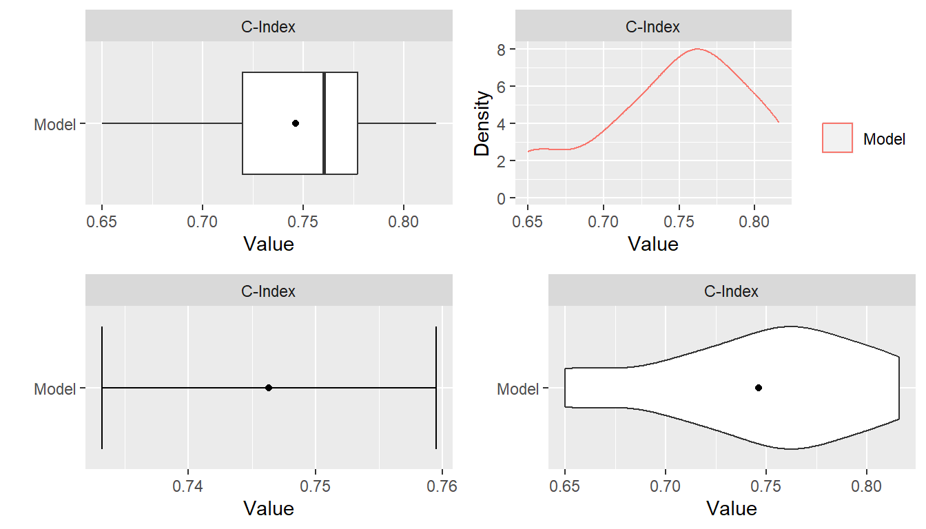
Stratified Resampling
Stratification of cases for the construction of resampled training
and test sets can be employed to help achieve balance across the sets.
Stratified resampling is automatically performed if variable
specification is in terms of a traditional formula or design matrix and
will be done according to the response variable. For model frames and
recipes, stratification variables must be defined explicitly with the
strata argument to the ModelFrame()
constructor or with the role_case()
function. In general, strata are constructed from numeric proportions
for BinomialVariate; original values for
character, factor, logical, and
ordered; first columns of values for matrix;
original values for numeric; and numeric times within event
statuses for Surv. Numeric values are stratified into
quantile bins and categorical values into factor levels defined by the
resampling control functions. Missing values are replaced with
non-missing values sampled at random with replacement.
## Model frame with response variable stratification
mf <- ModelFrame(surv_fo, data = surv_train, strata = surv_train$y)
resample(mf, model = GBMModel)

## Recipe with response variable stratification
rec <- recipe(y ~ ., data = surv_train) %>%
  role_case(stratum = y)
resample(rec, model = GBMModel)
Dynamic Model Parameters
As discussed previously in the Model Fit and Prediction section, dynamic model parameters are evaluated at the time of model fitting and can depend on the number of observations in the fitted dataset. In the context of resampling, dynamic parameters are repeatedly evaluated at each fit of the resampled datasets. As such, their values can change based on the observations selected for training at each iteration of the resampling algorithm.
## Dynamic model parameter k = log number of training set observations
resample(surv_fo, data = surv_train, model = CoxStepAICModel(k = .(log(nobs))))
Model Comparisons
Resampled metrics from different models can be combined for
comparison with the c()
function. Optional names given on the left hand side of equal operators
within c()
calls will be used as labels in output from the summary()
and plot()
functions. For comparisons of resampled output, the same control
structure must be used in all associated calls to resample()
to ensure that resulting model metrics are computed on the same
resampled training and test sets. The combined resample output can be
summarized and plotted as usual.
## Resample estimation
res1 <- resample(surv_fo, data = surv_train, model = GBMModel(n.trees = 25),
                 control = surv_means_control)
res2 <- resample(surv_fo, data = surv_train, model = GBMModel(n.trees = 50),
                 control = surv_means_control)
res3 <- resample(surv_fo, data = surv_train, model = GBMModel(n.trees = 100),
                 control = surv_means_control)

## Combine resample output for comparison
(res <- c(GBM1 = res1, GBM2 = res2, GBM3 = res3))
#> --- Resample object ---------------------------------------------------------
#>
#> Models: GBM1, GBM2, GBM3
#> Sampling variables:
#> # A tibble: 136 × 2
#>    Case  Stratification$`(strata)`
#>    <chr> <fct>
#>  1 159   0:(2.56e+03,3.45e+03]
#>  2 179   0:(3.45e+03,5.56e+03]
#>  3 14    1:[99,1.05e+03]
#>  4 195   0:(3.45e+03,5.56e+03]
#>  5 170   0:(2.56e+03,3.45e+03]
#>  6 50    0:[1.5e+03,1.92e+03]
#>  7 118   1:(1.05e+03,3.18e+03]
#>  8 43    1:(1.05e+03,3.18e+03]
#>  9 203   0:(3.45e+03,5.56e+03]
#> 10 199   0:(3.45e+03,5.56e+03]
#> # ℹ 126 more rows
#>
#> === CVControl object ===
#>
#> Label: K-Fold Cross-Validation
#> Folds: 5
#> Repeats: 3

summary(res)
#> , , Metric = C-Index
#>
#>       Statistic
#> Model       Mean    Median         SD       Min       Max NA
#>   GBM1 0.7748099 0.7951389 0.04746402 0.6497797 0.8301887  0
#>   GBM2 0.7647633 0.7630332 0.05151443 0.6497797 0.8632075  0
#>   GBM3 0.7463392 0.7601810 0.05087334 0.6497797 0.8160377  0

plot(res)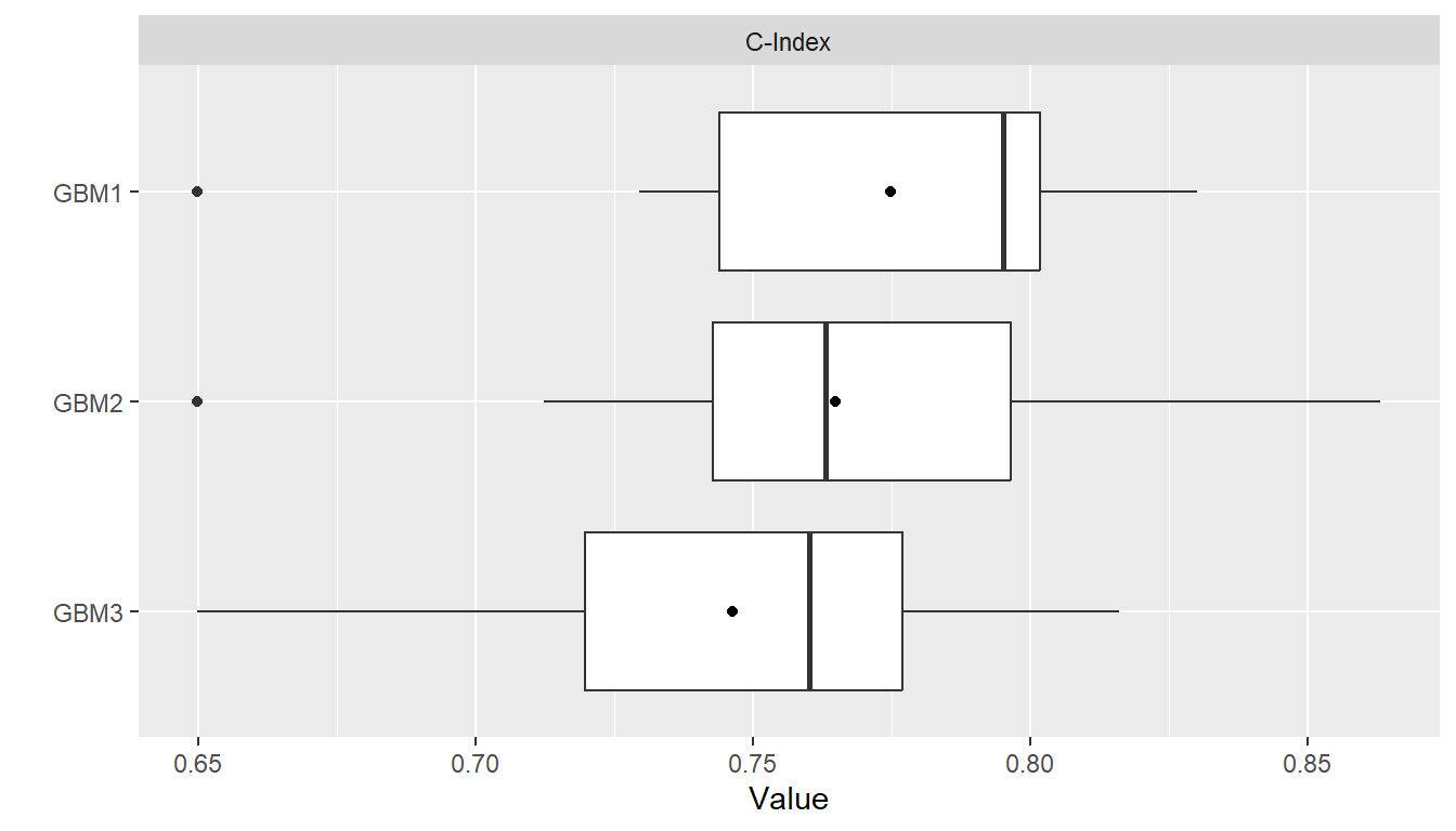
Pairwise model differences for each metric can be calculated with the
diff()
function applied to results from a call to c().
Resulting differences can be summarized descriptively with the summary()
and plot()
functions and assessed for statistical significance with pairwise
t-tests performed by the t.test()
function. The t-test statistic for a given set of \(R\) resampled differences is calculated as
\[
t = \frac{\bar{x}_R}{\sqrt{F s^2_R / R}},
\] where \(\bar{x}_R\) and \(s^2_R\) are the sample mean and variance.
Statistical testing for a mean difference is then performed by comparing
\(t\) to a \(t_{R-1}\) null distribution. The sample
variance in the t statistic is known to underestimate the true variances
of cross-validation mean estimators. Underestimation of these variances
will lead to increased probabilities of false-positive statistical
conclusions. Thus, an additional factor \(F\) is included in the t statistic to allow
for variance corrections. A correction of \(F
= 1 + K / (K - 1)\) was found by Nadeau and Bengio (2003) to be a good choice for cross-validation
with \(K\) folds and is thus used for
that resampling method. The extension of this correction by Bouchaert
and Frank (2004) to \(F = 1 + T K / (K - 1)\) is used for
cross-validation with \(K\) folds
repeated \(T\) times. For other
resampling methods \(F = 1\). Below are
t-test results based on the extended correction factor for 3 repeats of
5-fold cross-validation.
## Pairwise model comparisons
(res_diff <- diff(res))
#> --- PerformanceDiff object --------------------------------------------------
#>
#> Metric: C-Index
#> Models: GBM1 - GBM2, GBM1 - GBM3, GBM2 - GBM3
#>
#> === CVControl object ===
#>
#> Label: K-Fold Cross-Validation
#> Folds: 5
#> Repeats: 3

summary(res_diff)
#> , , Metric = C-Index
#>
#>              Statistic
#> Model               Mean     Median         SD          Min        Max NA
#>   GBM1 - GBM2 0.01004663 0.01388889 0.02165165 -0.033018868 0.03973510  0
#>   GBM1 - GBM3 0.02847075 0.02903226 0.02584321 -0.009803922 0.08293839  0
#>   GBM2 - GBM3 0.01842412 0.01376147 0.01974621  0.000000000 0.05743243  0

plot(res_diff)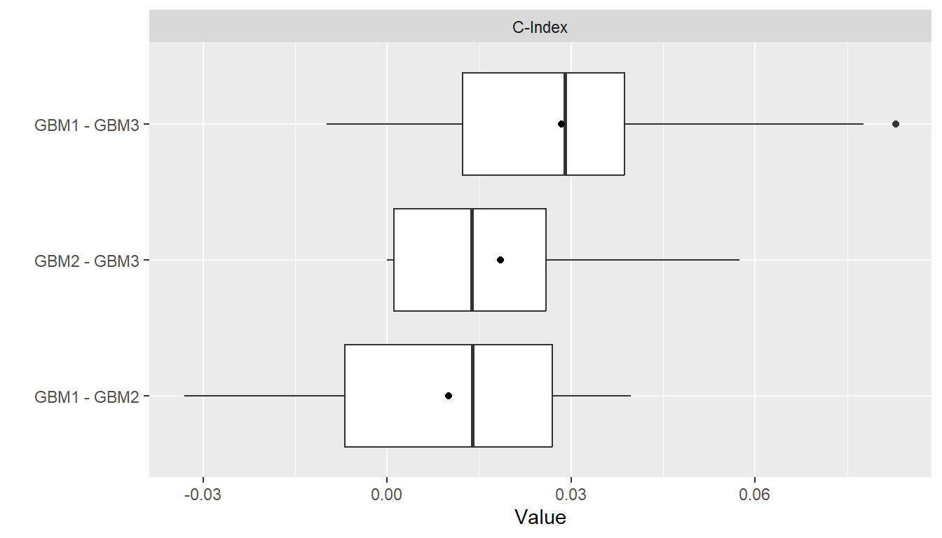
t.test(res_diff)
#> --- PerformanceDiffTest object ----------------------------------------------
#>
#> Upper diagonal: mean differences (Model1 - Model2)
#> Lower diagonal: p-values
#> P-value adjustment method: holm
#>
#> , , Metric = C-Index
#>
#>       Model2
#> Model1      GBM1       GBM2       GBM3
#>   GBM1        NA 0.01004663 0.02847075
#>   GBM2 0.4234417         NA 0.01842412
#>   GBM3 0.2115012 0.23906539         NA
Model Predictor Effects and Diagnostics
Calculation of performance metrics on test sets or by resampling, as discussed previously, is one method of assessing model performance. Others available include measures of predictor variable importance, partial dependence plots, calibration curves comparing observed and predicted response values, and receiver operating characteristic analysis.
Variable Importance
The importance of predictor variables in a model fit is estimated
with the varimp()
function and displayed graphically with plot().
Variable importance is a relative measure of the contributions of model
predictors and is scaled by default to have a maximum value of 100,
where higher values represent more important variables. Model-specific
implementations of variable importance are available in many cases,
although their definitions may differ. In the case of a GBMModel,
importance of each predictor is based on the sum of squared empirical
improvements over all internal tree nodes created by splitting on that
variable (Greenwell et al. 2019).
## Predictor variable importance
(vi <- varimp(surv_fit, method = "model"))
#> --- VariableImportance object -----------------------------------------------
#> Method: model
#> Metric: influence
#> Scale: 0.5524429
#> Values:
#>             Overall
#> age       100.00000
#> thickness  78.27486
#> year       45.60724
#> ulcer      26.88075
#> sex         8.93267

plot(vi)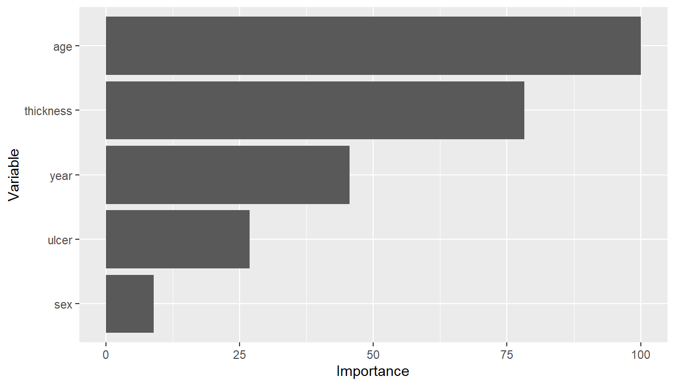
In contrast, importance is based on negative log-transformed p-values
for statistical models, like CoxModel,
that produce them. For other models, variable importance may be defined
and calculated by their underlying source packages or not defined at
all, as is the case for SVMModel.
Logical indicators of model-specific variable importance are given in
the information displayed by model constructors and returned by modelinfo().
SVMModel
#> --- MLModelFunction object --------------------------------------------------
#>
#> Model name: SVMModel
#> Label: Support Vector Machines
#> Package: kernlab
#> Response types: factor, numeric
#> Case weights support: FALSE
#> Missing case removal: all
#> Tuning grid: FALSE
#> Variable importance: FALSE
#>
#> Arguments:
#> function (scaled = TRUE, type = character(), kernel = c("rbfdot",
#>     "polydot", "vanilladot", "tanhdot", "laplacedot", "besseldot",
#>     "anovadot", "splinedot"), kpar = "automatic", C = 1, nu = 0.2,
#>     epsilon = 0.1, prob.model = FALSE, cache = 40, tol = 0.001,
#>     shrinking = TRUE)
#> NULL

modelinfo(SVMModel)[[1]]$varimp
#> [1] FALSE
Variable importance can be computed with model-agnostic permutation methods (Fisher et al. 2019) as an alternative to model-specific methods. The following algorithm for permutation-based variable importance is implemented and the default method in MachineShop.
Fit a model to a training dataset.
Compute training performance.
For \(s = 1, \ldots, S\).
Optionally sample a subset of the training set without replacement.
For predictor variable \(p = 1, \ldots, P\).
Randomly permute the variable values.
Compute performance on the permutation set.
Compute importance as the difference or ratio between the permutation and training performances.
Reset the variable to its original values.
Return the mean or other summary statistics of importance for each variable.
## Permutation-based variable importance
varimp(surv_fit)
#> --- VariableImportance object -----------------------------------------------
#> Method: permute
#> Metric: cindex
#> Scale: 0.0007956676
#> Values:
#>                 Mean
#> age       100.000000
#> thickness  90.837696
#> ulcer      69.371728
#> year       50.130890
#> sex         6.151832
There are a number of advantages to permutation-based variable importance. In particular, it can be computed for any
- model,
- performance metric defined for the given response variable type, and
- predictor variable in the original training set.
Conversely, model-specific methods are not defined for some models, are generally limited to metrics implemented in their source packages, and might be computed on derived, rather than original, predictor variables. These differences can make comparisons of variable importance across classes of models difficult if not impossible. The trade-off for the advantages of a permutation-based approach is increased computation time. To speed up computations, the algorithm will run in parallel if a compatible backend is loaded as described in the Parallel Processing section.
Recursive Feature Elimination
Recursive feature elimination (RFE) is a wrapper method of variable
selection. In wrapper methods, a given model is fit to subsets of
predictor variables in order to select the subset whose fit is optimal.
Forward, backward, and step-wise variable selection are examples of
wrapper methods. RFE is a type of backward selection in which subsets
are formed from decreasing numbers of the most important predictor
variables. The RFE algorithm implemented in the package-supplied
rfe() function is summarized below.
Compute variable importance for all predictors.
For predictor subsets of sizes \(S = S_n > ... > S_1\).
Eliminate predictors whose variable importance is not in the top \(S\) by randomly permuting their values.
Compute a resampled estimate of model predictive performance.
Optionally recompute variable importance for the top \(S\) predictors, and set importance equal to zero for those eliminated.
Select the predictor set with highest predictive performance.
This RFE algorithm differs from others in that variables are
“eliminated” by permuting their values rather than by removing them from
the dataset. Using a permutation approach for both the elimination of
variables and computation of variable importance enables application of
the rfe() function to any variable specification
(traditional formula, design matrix, model frame, or recipe) and any
model available in the package. The syntax for rfe() is
similar to resample() as illustrated in the following
example.
## Recursive feature elimination
(surv_rfe <- rfe(surv_fo, data = surv_train, model = GBMModel,
                 control = surv_means_control))
#> --- TrainingStep object -----------------------------------------------------
#>
#> Optimization method: Global Recursive Feature Elimination
#> ModelSpecification log:
#> # A tibble: 4 × 5
#>   name                 terms     selected params$size metrics$`C-Index`
#>   <chr>                <list>    <lgl>          <int>             <dbl>
#> 1 ModelSpecification.1 <chr [5]> FALSE              5             0.746
#> 2 ModelSpecification.2 <chr [4]> FALSE              4             0.736
#> 3 ModelSpecification.3 <chr [2]> TRUE               2             0.748
#> 4 ModelSpecification.4 <chr [1]> FALSE              1             0.701
#>
#> Selected row: 3
#> Metric: C-Index = 0.7481588
rfe_summary <- summary(surv_rfe)
rfe_summary$terms[rfe_summary$selected]
#> [[1]]
#> [1] "age"       "thickness"
Partial Dependence Plots
Partial dependence plots show the marginal effects of predictors on a response variable. Dependence for a select set of one or more predictor variables \(X_S\) is computed as \[ \bar{f}_S(X_S) = \frac{1}{N}\sum_{i=1}^N f(X_S, x_{iS'}), \] where \(f\) is a fitted prediction function and \(x_{iS'}\) are values of the remaining predictors in a dataset of \(N\) cases. The response scale displayed in dependence plots will depend on the response variable type: probability for predicted factors and survival probabilities, original scale for numerics, and survival time for predicted survival means. By default, dependence is computed for each selected predictor individually over a grid of 10 approximately evenly spaced values and averaged over the dataset on which the prediction function was fit.
## Partial dependence plots
pd <- dependence(surv_fit, select = c(thickness, age))
plot(pd)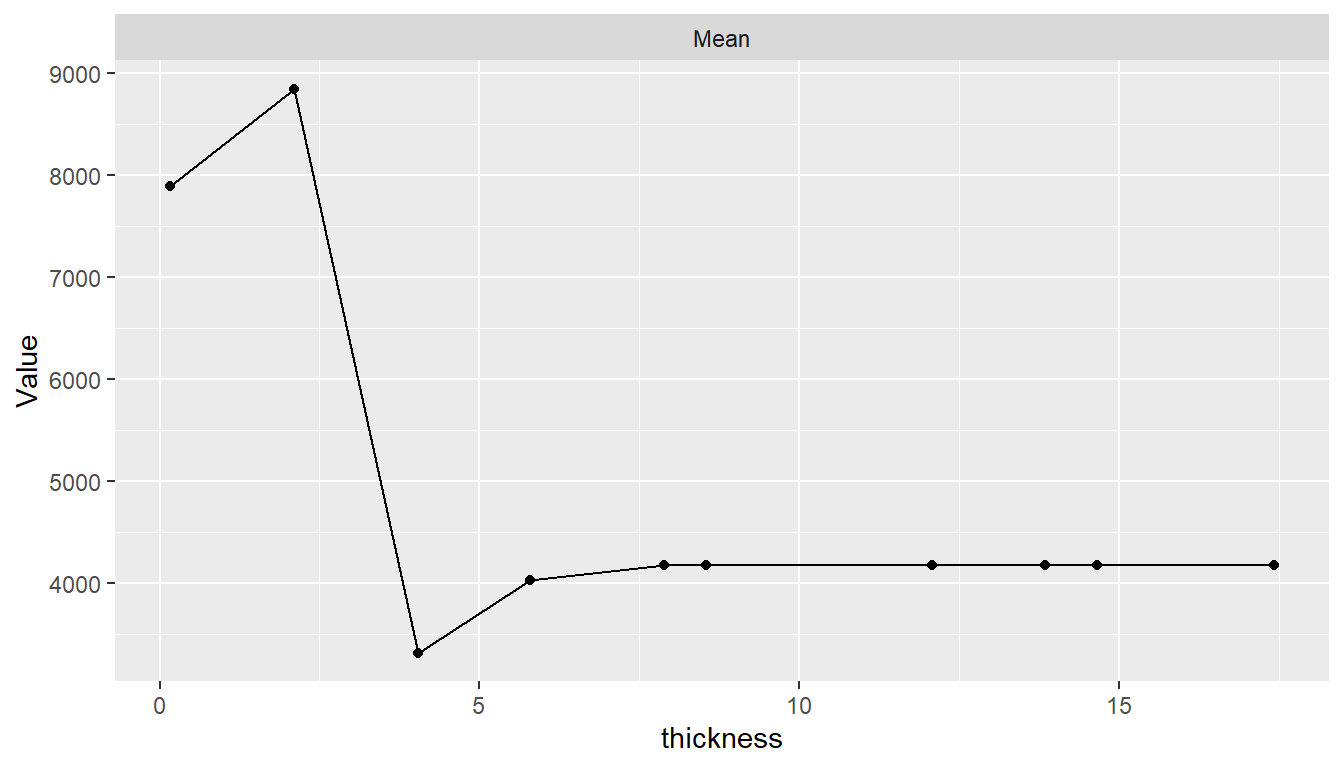
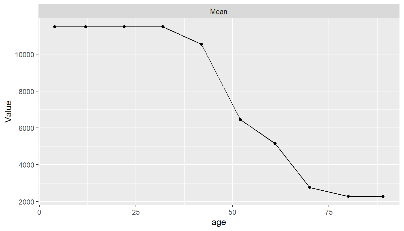
Estimated predictor effects are marginal in that they are averaged over the remaining variables, whose distribution depends on the population represented by the dataset. Consequently, partial dependence plots for a given model can vary across datasets and populations. The package allows averaging over different datasets to estimate marginal effects in other case populations, over different numbers of predictor values, and over quantile spacing of the values.
pd <- dependence(surv_fit, data = surv_test, select = thickness, n = 20,
                 intervals = "quantile")
plot(pd)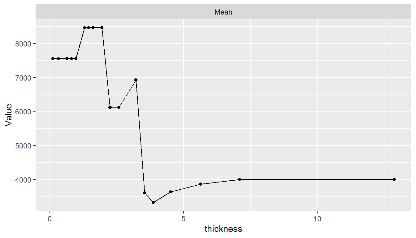
In addition, dependence may be computed for combinations of multiple predictors to examine interaction effects and for summary statistics other than the mean.
Calibration Curves
Agreement between model-predicted and observed values can be visualized with calibration curves. Calibration curves supplement individual performance metrics with information on model fit in different regions of predicted values. They also provide more direct assessment of agreement than some performance metrics, like ROC AUC, that do not account for scale and location differences. In the construction of binned calibration curves, cases are partitioned into equal-width intervals according to their (resampled) predicted responses. Mean observed responses are then calculated within each of the bins and plotted on the vertical axis against the bin midpoints on the horizontal axis.
## Binned calibration curves
cal <- calibration(res_probs, breaks = 10)
plot(cal, se = TRUE)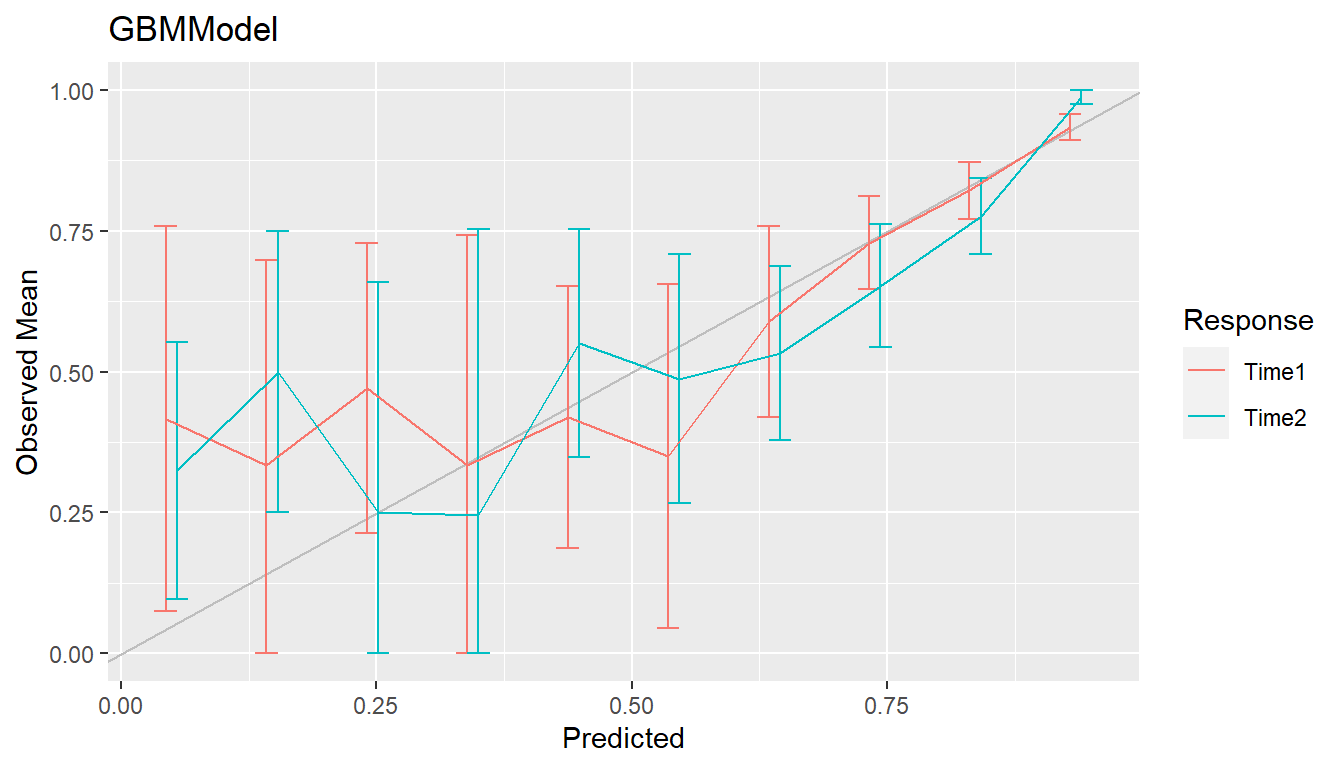
As an alternative to discrete bins, curves can be smoothed by setting
breaks = NULL to compute weighted averages of observed
values. Smoothing has the advantage of producing more precise curves by
including more observed values in the calculation at each predicted
value.
## Smoothed calibration curves
cal <- calibration(res_probs, breaks = NULL)
plot(cal, se = TRUE)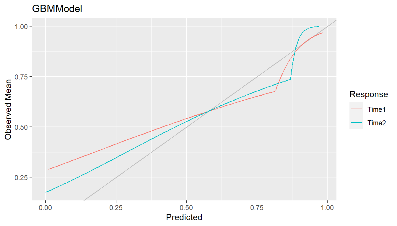
Calibration curves close to the 45\(^\circ\) line represent agreement between observed and predicted responses and a model that is said to be well calibrated.
Confusion Matrices
Confusion matrices of cross-classified observed and predicted
categorical responses are available with the confusion()
function. They can be constructed with predicted class membership or
with predicted class probabilities. In the latter case, predicted class
membership is derived from predicted probabilities according to a
probability cutoff value for binary factors (default:
cutoff = 0.5) and according to the class with highest
probability for factors with more than two levels.
## Confusion matrices
(conf <- confusion(res_probs, cutoff = 0.7))
#> --- ConfusionList object ----------------------------------------------------
#>
#> === $GBMModel.Time1 =========================================================
#> === BinaryConfusionMatrix object ===
#>          Observed
#> Predicted         0         1
#>         0 236.02496  38.97504
#>         1  59.34328  73.65672
#>
#> === $GBMModel.Time2 =========================================================
#> === BinaryConfusionMatrix object ===
#>          Observed
#> Predicted         0         1
#>         0 170.20031  34.79969
#>         1  82.12352 120.87648
plot(conf)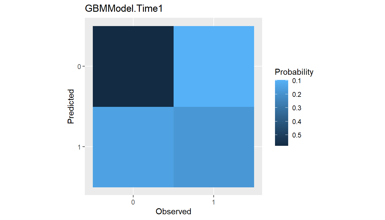
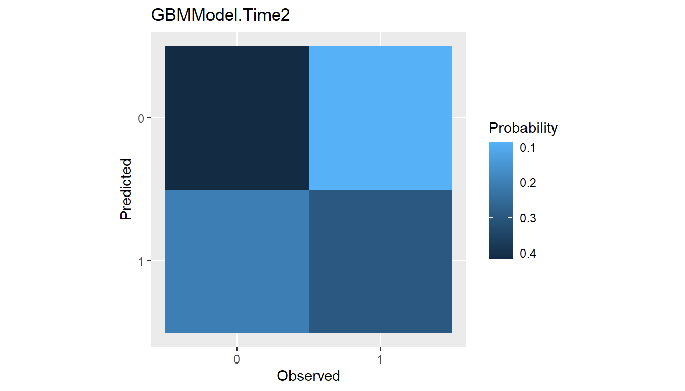
Confusion matrices are the data structure upon which many of the
performance metrics described earlier for factor predictor variables are
based. Metrics commonly reported for confusion matrices are generated by
the summary()
function.
## Summary performance metrics
summary(conf)
#> --- $GBMModel.Time1 ---------------------------------------------------------
#> Number of responses: 408
#> Accuracy (SE): 0.7590237 (0.02117311)
#> Majority class: 0.7239418
#> Kappa: 0.4290466
#>
#>                     0         1
#> Observed    0.7239418 0.2760582
#> Predicted   0.6740196 0.3259804
#> Agreement   0.5784925 0.1805312
#> Sensitivity 0.7990871 0.6539605
#> Specificity 0.6539605 0.7990871
#> PPV         0.8582726 0.5538099
#> NPV         0.5538099 0.8582726
#>
#> --- $GBMModel.Time2 ---------------------------------------------------------
#> Number of responses: 408
#> Accuracy (SE): 0.7134235 (0.02238535)
#> Majority class: 0.6184408
#> Kappa: 0.4261807
#>
#>                     0         1
#> Observed    0.6184408 0.3815592
#> Predicted   0.5024510 0.4975490
#> Agreement   0.4171576 0.2962659
#> Sensitivity 0.6745312 0.7764610
#> Specificity 0.7764610 0.6745312
#> PPV         0.8302454 0.5954506
#> NPV         0.5954506 0.8302454
Summaries can also be obtained with the performance()
function for default or use-specified metrics.
## Confusion matrix-specific metrics
metricinfo(conf) %>% names
#>  [1] "accuracy"    "f_score"     "fnr"         "fpr"         "kappa2"
#>  [6] "npv"         "ppr"         "ppv"         "precision"   "recall"
#> [11] "roc_index"   "sensitivity" "specificity" "tnr"         "tpr"

## User-specified metrics
performance(conf, metrics = c("Accuracy" = accuracy,
                              "Sensitivity" = sensitivity,
                              "Specificity" = specificity))
#> --- $GBMModel.Time1 ---------------------------------------------------------
#>    Accuracy Sensitivity Specificity
#>   0.7590237   0.6539605   0.7990871
#>
#> --- $GBMModel.Time2 ---------------------------------------------------------
#>    Accuracy Sensitivity Specificity
#>   0.7134235   0.7764610   0.6745312
Performance Curves
Tradeoffs between correct and incorrect classifications of binary responses, across the range of possible cutoff probabilities, can be studied with performance curves. In general, any two binary response metrics may be specified for the construction of a performance curve.
ROC Curves
Receiver operating characteristic (ROC) curves are one example in which true positive rates (sensitivity) are plotted against false positive rates (1 - specificity) (Fawcett 2006). True positive rate (TPR) and false positive rate (FPR) are defined as \[ \begin{aligned} TPR &= \text{sensitivity} = \Pr(\hat{p} > c \mid D^+) \\ FPR &= 1 - \text{specificity} = \Pr(\hat{p} > c \mid D^-), \end{aligned} \] where \(\hat{p}\) is the model-predicted probability of being positive, \(0 \le c \le 1\) is a probability cutoff value for classification as positive or negative, and \(D^+/D^-\) is positive/negative case status. ROC curves show tradeoffs between the two rates over the range of possible cutoff values. Higher curves are indicative of better predictive performance.
## ROC curves
roc <- performance_curve(res_probs)
plot(roc, diagonal = TRUE)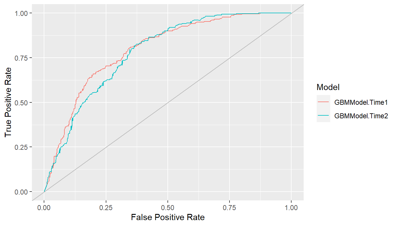
ROC curves show the relation between the two rates being plotted but
not their relationships with specific cutoff values. The latter may be
helpful for the selection of a cutoff to apply in practice. Accordingly,
separate plots of each rate versus the range of possible cutoffs are
available with the type = "cutoffs" option.
plot(roc, type = "cutoffs")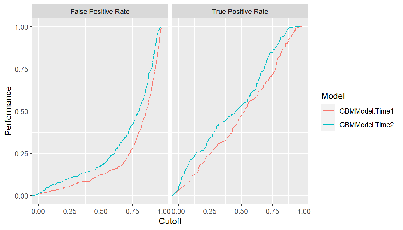
Area under the ROC curve (ROC AUC) is an overall measure of model predictive performance. It is interpreted as the probability that a randomly selected positive case will have a higher predicted value than a randomly selected negative case. AUC values of 0.5 and 1.0 indicate chance and perfect concordance between predicted probabilities and observed responses.
auc(roc)
#> Model: GBMModel.Time1
#> [1] 0.7966402
#> ------------------------------------------------------------
#> Model: GBMModel.Time2
#> [1] 0.7818386
Precision Recall Curves
Precision recall curves plot precision (positive predictive value) against recall (sensitivity) (Davis and Goadrich 2006), where \[ \begin{aligned} \text{precision} &= PPV = \Pr(D^+ \mid \hat{p} > c) \\ \text{recall} &= \text{sensitivity} = \Pr(\hat{p} > c \mid D^+). \end{aligned} \] These curves tend to be used when primary interest lies in detecting positive cases and such cases are rare.
## Precision recall curves
pr <- performance_curve(res_probs, metrics = c(precision, recall))
plot(pr)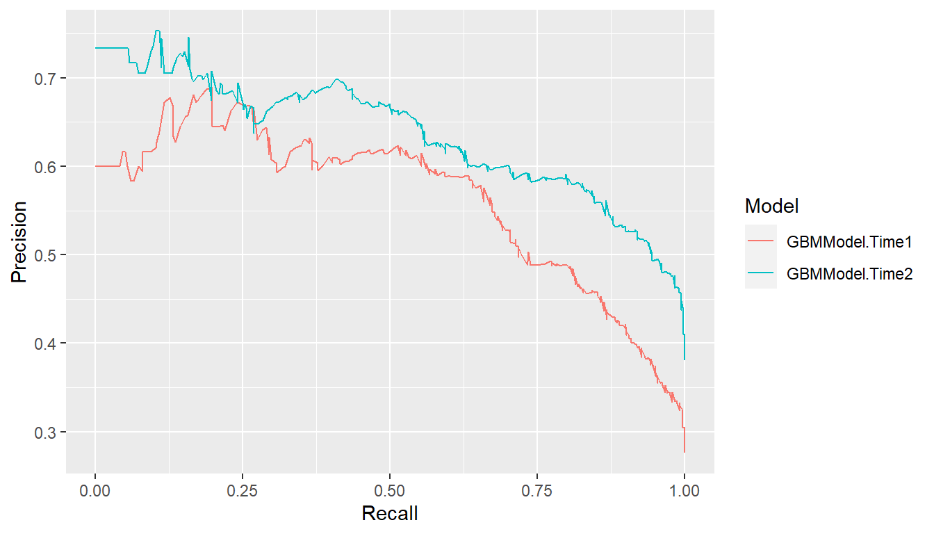
auc(pr)
#> Model: GBMModel.Time1
#> [1] 0.562425
#> ------------------------------------------------------------
#> Model: GBMModel.Time2
#> [1] 0.6359023
Lift Curves
Lift curves depict the rate at which positive cases are found as a function of the proportion predicted to be positive in the population. In particular, they plot true positive rate (sensitivity) against positive prediction rate (PPR) for all possible classification probability cutoffs, where \[ \begin{aligned} TPR &= \Pr(\hat{p} > c \mid D^+) \\ PPR &= \Pr(\hat{p} > c). \end{aligned} \] Models more efficient (lower cost) at identifying positive cases find them at a higher proportion (\(TPR\)) while predicting fewer in the overall population to be positive (\(PPR\)). In other words, higher lift curves are signs of model efficiency.
## Lift curves
lf <- lift(res_probs)
plot(lf, find = 0.75)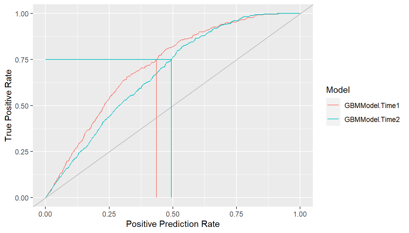
Modeling Strategies
Model development often involves the comparison of multiple models from a candidate set for the purpose of selecting a final one. Models in the set may differ with respect to their predictor variables, preprocessing steps and parameters, and model types and parameters. Complex model selection strategies for sets that involve one or more of these differences can be implemented with the MachineShop package. Implementation is achieved with a straightforward syntax based on the meta-input and meta-model functions listed in the table below and with resampling, including nested resampling, conducted automatically for model selection and predictive performance evaluation.
| Parameter Grid Tuning | Candidate Set Selection | Ensemble Learning |
|---|---|---|
TunedInput() |
SelectedInput() |
StackedModel() |
TunedModel() |
SelectedModel() |
SuperModel() |
These meta-functions fall into three main categories: 1) tuning of a
given input or model over a grid of parameter values, 2) selection from
an arbitrary set of different inputs or models, or 3) combining multiple
models into an ensemble learner. In the context of these strategies, an
input may be a formula, design matrix, model frame, or preprocessing
recipe. The meta-input and meta-model functions themselves return input
and model class objects, respectively. Combinations and multiple levels
of nesting of meta-functions, inputs, and models are allowed. For
example, StackedModel()
and SuperModel()
may consist of TunedModel
and other model objects. SelectedModel()
can select among mixes of TunedModel,
ensemble model, and other model objects. Likewise, TunedInput
objects, along with other inputs, may be nested within SelectedInput().
Furthermore, selection and tuning of both inputs and models can be
performed simultaneously. These and other possibilities are illustrated
in the following sections.
Inputs
Inputs to model fitting functions define the predictor and response variables and the dataset containing their values. These can be specified with traditional formula and dataset pairs, design matrix and response variable pairs, model frames, and preprocessing recipes. The package supports (1) tuning of an input over a grid of parameter values and (2) selection of inputs from candidate sets that differ with respect to their predictors or their preprocessing steps and parameters.
Input Tuning
Preprocessing recipes may have step with parameters that affect
predictive performance. Steps can be tuned over a grid of parameter
values with TunedInput()
to select the best performing values. Calls to TunedInput()
return an input object that may be trained on data with the fit()
function or evaluated for predictive performance with resample().
As an example, a principal components analysis (PCA) step could be
included in a preprocessing recipe for tuning over the number of
components to retain in the final model. Such a recipe is shown below
accompanied by a call to expand_steps()
to construct a tuning grid. The grid parameter num_comp and
name PCA correspond to the argument and id of the step_pca()
function to which the values 1:3 apply. The recipe and grid
may then be passed to TunedInput()
for model fitting.
## Preprocessing recipe with PCA steps
pca_rec <- recipe(y ~ ., data = surv_train) %>%
  role_case(stratum = y) %>%
  step_center(all_predictors()) %>%
  step_scale(all_predictors()) %>%
  step_pca(all_predictors(), id = "PCA")

## Tuning grid of number of PCA components
pca_grid <- expand_steps(
  PCA = list(num_comp = 1:3)
)

## Tuning specification
tun_rec <- TunedInput(pca_rec, grid = pca_grid)
From the fit, the resulting model can be extracted with as.MLModel().
The output shows that one principal component was selected. Resample
estimation of predictive performance is applied to a TunedInput
specification for the selection. The default resampling method is
cross-validation. Other methods, performance metrics, and selection
statistics can be supplied to the TunedInput()
arguments.
## Input-tuned model fit and final trained model
model_fit <- fit(tun_rec, model = GBMModel)
as.MLModel(model_fit)
#> --- MLModel object ----------------------------------------------------------
#>
#> Model name: GBMModel
#> Label: Trained Generalized Boosted Regression
#> Package: gbm
#> Response types: factor, numeric, PoissonVariate, Surv
#> Case weights support: TRUE
#> Missing case removal: response
#> Tuning grid: TRUE
#> Variable importance: TRUE
#>
#> Parameters:
#> List of 5
#>  $ n.trees          : num 100
#>  $ interaction.depth: num 1
#>  $ n.minobsinnode   : num 10
#>  $ shrinkage        : num 0.1
#>  $ bag.fraction     : num 0.5
#>
#> === $TrainingStep1 ==========================================================
#> === TrainingStep object ===
#>
#> Optimization method: Grid Search
#> TunedModelRecipe log:
#> # A tibble: 3 × 4
#>   name          selected params$PCA$num_comp metrics$`C-Index`
#>   <chr>         <lgl>                  <int>             <dbl>
#> 1 ModelRecipe.1 TRUE                       1             0.740
#> 2 ModelRecipe.2 FALSE                      2             0.720
#> 3 ModelRecipe.3 FALSE                      3             0.725
#>
#> Selected row: 1
#> Metric: C-Index = 0.7399641
Input Selection
Selection of recipes with different steps or predictors can be
conducted with SelectedInput().
## Preprocessing recipe without PCA steps
rec1 <- recipe(y ~ sex + age + year + thickness + ulcer, data = surv_train) %>%
  role_case(stratum = y)
rec2 <- recipe(y ~ sex + age + year, data = surv_train) %>%
  role_case(stratum = y)

## Selection among recipes with and without PCA steps
sel_rec <- SelectedInput(
  rec1,
  rec2,
  TunedInput(pca_rec, grid = pca_grid)
)
In this case, the third recipe with PCA steps is selected.
## Input-selected model fit and model
model_fit <- fit(sel_rec, model = GBMModel)
as.MLModel(model_fit)
#> --- MLModel object ----------------------------------------------------------
#>
#> Model name: GBMModel
#> Label: Trained Generalized Boosted Regression
#> Package: gbm
#> Response types: factor, numeric, PoissonVariate, Surv
#> Case weights support: TRUE
#> Missing case removal: response
#> Tuning grid: TRUE
#> Variable importance: TRUE
#>
#> Parameters:
#> List of 5
#>  $ n.trees          : num 100
#>  $ interaction.depth: num 1
#>  $ n.minobsinnode   : num 10
#>  $ shrinkage        : num 0.1
#>  $ bag.fraction     : num 0.5
#>
#> === $TrainingStep1 ==========================================================
#> === TrainingStep object ===
#>
#> Optimization method: Grid Search
#> SelectedModelRecipe log:
#> # A tibble: 3 × 4
#>   name             selected params$id  metrics$`C-Index`
#>   <chr>            <lgl>    <chr>                  <dbl>
#> 1 ModelRecipe.1    FALSE    input.azpi             0.761
#> 2 ModelRecipe.2    FALSE    input.aLHo             0.643
#> 3 TunedModelRecipe TRUE     input.W4KN             0.796
#>
#> Selected row: 3
#> Metric: C-Index = 0.7960841
#>
#> === $TrainingStep2 ==========================================================
#> === TrainingStep object ===
#>
#> Optimization method: Grid Search
#> TunedModelRecipe log:
#> # A tibble: 3 × 4
#>   name          selected params$PCA$num_comp metrics$`C-Index`
#>   <chr>         <lgl>                  <int>             <dbl>
#> 1 ModelRecipe.1 TRUE                       1             0.740
#> 2 ModelRecipe.2 FALSE                      2             0.720
#> 3 ModelRecipe.3 FALSE                      3             0.725
#>
#> Selected row: 1
#> Metric: C-Index = 0.7399641
Selection can also be performed among traditional formulas, design matrices, or model frames.
## Traditional formulas
fo1 <- y ~ sex + age + year + thickness + ulcer
fo2 <- y ~ sex + age + year

## Selection among formulas
sel_fo <- SelectedInput(fo1, fo2, data = surv_train)

## Input-selected model fit and final trained model
model_fit <- fit(sel_fo, model = GBMModel)
as.MLModel(model_fit)
#> --- MLModel object ----------------------------------------------------------
#>
#> Model name: GBMModel
#> Label: Trained Generalized Boosted Regression
#> Package: gbm
#> Response types: factor, numeric, PoissonVariate, Surv
#> Case weights support: TRUE
#> Missing case removal: response
#> Tuning grid: TRUE
#> Variable importance: TRUE
#>
#> Parameters:
#> List of 5
#>  $ n.trees          : num 100
#>  $ interaction.depth: num 1
#>  $ n.minobsinnode   : num 10
#>  $ shrinkage        : num 0.1
#>  $ bag.fraction     : num 0.5
#>
#> === $TrainingStep1 ==========================================================
#> === TrainingStep object ===
#>
#> Optimization method: Grid Search
#> SelectedModelFrame log:
#> # A tibble: 2 × 4
#>   name         selected params$id  metrics$`C-Index`
#>   <chr>        <lgl>    <chr>                  <dbl>
#> 1 ModelFrame.1 TRUE     input.CuYF             0.745
#> 2 ModelFrame.2 FALSE    input.W4KN             0.664
#>
#> Selected row: 1
#> Metric: C-Index = 0.7452425
In the previous examples, selection of different inputs was performed
with the same model (GBMModel).
Selection among different combinations of inputs and models is supported
with the ModelSpecification()
constructor.
## Different combinations of inputs and models
sel_mfo <- SelectedInput(
  ModelSpecification(fo1, data = surv_train, model = CoxModel),
  ModelSpecification(fo2, data = surv_train, model = GBMModel)
)

## Input-selected model fit and final trained model
model_fit <- fit(sel_mfo)
as.MLModel(model_fit)
#> --- MLModel object ----------------------------------------------------------
#>
#> Model name: CoxModel
#> Label: Trained Cox Regression
#> Package: survival
#> Response type: Surv
#> Case weights support: TRUE
#> Missing case removal: all
#> Tuning grid: FALSE
#> Variable importance: TRUE
#>
#> Parameter:
#> List of 1
#>  $ ties: chr "efron"
#>
#> === $TrainingStep1 ==========================================================
#> === TrainingStep object ===
#>
#> Optimization method: Grid Search
#> SelectedModelSpecification log:
#> # A tibble: 2 × 4
#>   name                 selected params$id  metrics$`C-Index`
#>   <chr>                <lgl>    <chr>                  <dbl>
#> 1 ModelSpecification.1 TRUE     mspec.azpi             0.783
#> 2 ModelSpecification.2 FALSE    mspec.80bs             0.664
#>
#> Selected row: 1
#> Metric: C-Index = 0.7829086
Models
Models define the functional relationships between predictor and response variables from a given set of inputs.
Model Tuning
Many of the package-supplied modeling functions have arguments, or
tuning parameters, that control aspects of their model fitting
algorithms. For example, GBMModel
parameters n.trees and interaction.depth
control the number of decision trees to fit and the maximum tree depths.
When called with a TunedModel,
the fit()
function performs model fitting over a grid of parameter values and
returns the model with the optimal values. Optimality is determined
based on the first performance metric of the metrics
argument to TunedModel()
if given or the first default metric of the performance()
function otherwise. Argument grid additionally controls the
construction of grid values and can be a single integer or vector of
integers whose positions or names match the parameters in a model’s
pre-defined tuning grid if one exists and which specify the number of
values used to construct the grid. Pre-defined TunedModel
grids can be extract and viewed apart from model fitting with expand_modelgrid().
As shown in the output below, as.MLModel()
will extract a tuned model from fit results for viewing of the tuning
parameter grid values, the names of models fit to each, all calculated
metrics, the final model selected, the metric upon which its selection
was based, and its parameters.
## Tune over automatic grid of model parameters
model_fit <- fit(surv_fo, data = surv_train,
                 model = TunedModel(
                   GBMModel,
                   grid = 3,
                   control = surv_means_control,
                   metrics = c("CIndex" = cindex, "RMSE" = rmse)
                 ))
(trained_model <- as.MLModel(model_fit))
#> --- MLModel object ----------------------------------------------------------
#>
#> Model name: GBMModel
#> Label: Trained Generalized Boosted Regression
#> Package: gbm
#> Response types: factor, numeric, PoissonVariate, Surv
#> Case weights support: TRUE
#> Missing case removal: response
#> Tuning grid: TRUE
#> Variable importance: TRUE
#>
#> Parameters:
#> List of 5
#>  $ n.trees          : int 50
#>  $ interaction.depth: int 1
#>  $ n.minobsinnode   : num 10
#>  $ shrinkage        : num 0.1
#>  $ bag.fraction     : num 0.5
#>
#> === $TrainingStep1 ==========================================================
#> === TrainingStep object ===
#>
#> Optimization method: Grid Search
#> TunedModel log:
#> # A tibble: 9 × 4
#>   name       selected params$n.trees $interaction.depth metrics$CIndex  $RMSE
#>   <chr>      <lgl>             <int>              <int>          <dbl>  <dbl>
#> 1 GBMModel.1 TRUE                 50                  1          0.765  3869.
#> 2 GBMModel.2 FALSE                50                  2          0.750  5450.
#> 3 GBMModel.3 FALSE                50                  3          0.739  7877.
#> 4 GBMModel.4 FALSE               100                  1          0.746  3919.
#> 5 GBMModel.5 FALSE               100                  2          0.730  5262.
#> 6 GBMModel.6 FALSE               100                  3          0.720 10596.
#> 7 GBMModel.7 FALSE               150                  1          0.726  4167.
#> 8 GBMModel.8 FALSE               150                  2          0.712  5428.
#> 9 GBMModel.9 FALSE               150                  3          0.699 16942.
#>
#> Selected row: 1
#> Metric: CIndex = 0.7647633
Grid values may also be given as a TuningGrid
function, function name, or object; ParameterGrid
object; or data frame containing parameter values at which to evaluate
the model, such as that returned by expand_params().
## Tune over randomly sampled grid points
fit(surv_fo, data = surv_train,
    model = TunedModel(
      GBMModel,
      grid = TuningGrid(size = 100, random = 10),
      control = surv_means_control
    ))

## Tune over user-specified grid points
fit(surv_fo, data = surv_train,
    model = TunedModel(
      GBMModel,
      grid = expand_params(
        n.trees = c(25, 50, 100),
        interaction.depth = 1:3
      ),
      control = surv_means_control
    ))
Statistics summarizing the resampled performance metrics across all
tuning parameter combinations can be obtained with the summary()
and performance()functions.
summary(trained_model)
#> --- $TrainingStep1 ----------------------------------------------------------
#> # A tibble: 9 × 4
#>   name       selected params$n.trees $interaction.depth metrics$CIndex  $RMSE
#>   <chr>      <lgl>             <int>              <int>          <dbl>  <dbl>
#> 1 GBMModel.1 TRUE                 50                  1          0.765  3869.
#> 2 GBMModel.2 FALSE                50                  2          0.750  5450.
#> 3 GBMModel.3 FALSE                50                  3          0.739  7877.
#> 4 GBMModel.4 FALSE               100                  1          0.746  3919.
#> 5 GBMModel.5 FALSE               100                  2          0.730  5262.
#> 6 GBMModel.6 FALSE               100                  3          0.720 10596.
#> 7 GBMModel.7 FALSE               150                  1          0.726  4167.
#> 8 GBMModel.8 FALSE               150                  2          0.712  5428.
#> 9 GBMModel.9 FALSE               150                  3          0.699 16942.

performance(trained_model) %>% lapply(summary)
#> $TrainingStep1
#> , , Metric = CIndex
#>
#>             Statistic
#> Model             Mean    Median         SD       Min       Max NA
#>   GBMModel.1 0.7647633 0.7630332 0.05151443 0.6497797 0.8632075  0
#>   GBMModel.2 0.7502765 0.7549020 0.04636802 0.6688742 0.8349057  0
#>   GBMModel.3 0.7388766 0.7500000 0.04594197 0.6621622 0.8197425  0
#>   GBMModel.4 0.7463392 0.7601810 0.05087334 0.6497797 0.8160377  0
#>   GBMModel.5 0.7301734 0.7345133 0.04361416 0.6621622 0.7847222  0
#>   GBMModel.6 0.7199483 0.7122642 0.05168649 0.6216216 0.7889908  0
#>   GBMModel.7 0.7263693 0.7385321 0.05069831 0.6351351 0.7896996  0
#>   GBMModel.8 0.7121314 0.7169811 0.05331152 0.6199095 0.7847222  0
#>   GBMModel.9 0.6994678 0.7156863 0.05314909 0.6081081 0.7639485  0
#>
#> , , Metric = RMSE
#>
#>             Statistic
#> Model             Mean    Median        SD      Min       Max NA
#>   GBMModel.1  3868.629  3321.249  1431.839 2123.875  7401.789  0
#>   GBMModel.2  5450.093  4741.129  2438.173 2385.426 11695.273  0
#>   GBMModel.3  7877.487  5827.739  5036.837 4192.463 20009.854  0
#>   GBMModel.4  3919.126  3535.514  1454.999 2373.413  7558.280  0
#>   GBMModel.5  5262.122  5052.969  1900.353 2280.193  8212.727  0
#>   GBMModel.6 10595.888  8308.733  7057.327 4996.420 28610.367  0
#>   GBMModel.7  4167.128  3789.596  1115.371 2587.440  6701.087  0
#>   GBMModel.8  5427.518  6129.309  2313.742 2039.894  9212.369  0
#>   GBMModel.9 16941.696 10865.160 16841.774 4914.743 71150.177  0
Line plots of tuning results display the resampled metric means, or
another statistic specified with the stat argument, versus
the first tuning parameter values and with lines grouped according to
the remaining parameters, if any.
plot(trained_model, type = "line")
#> $TrainStep1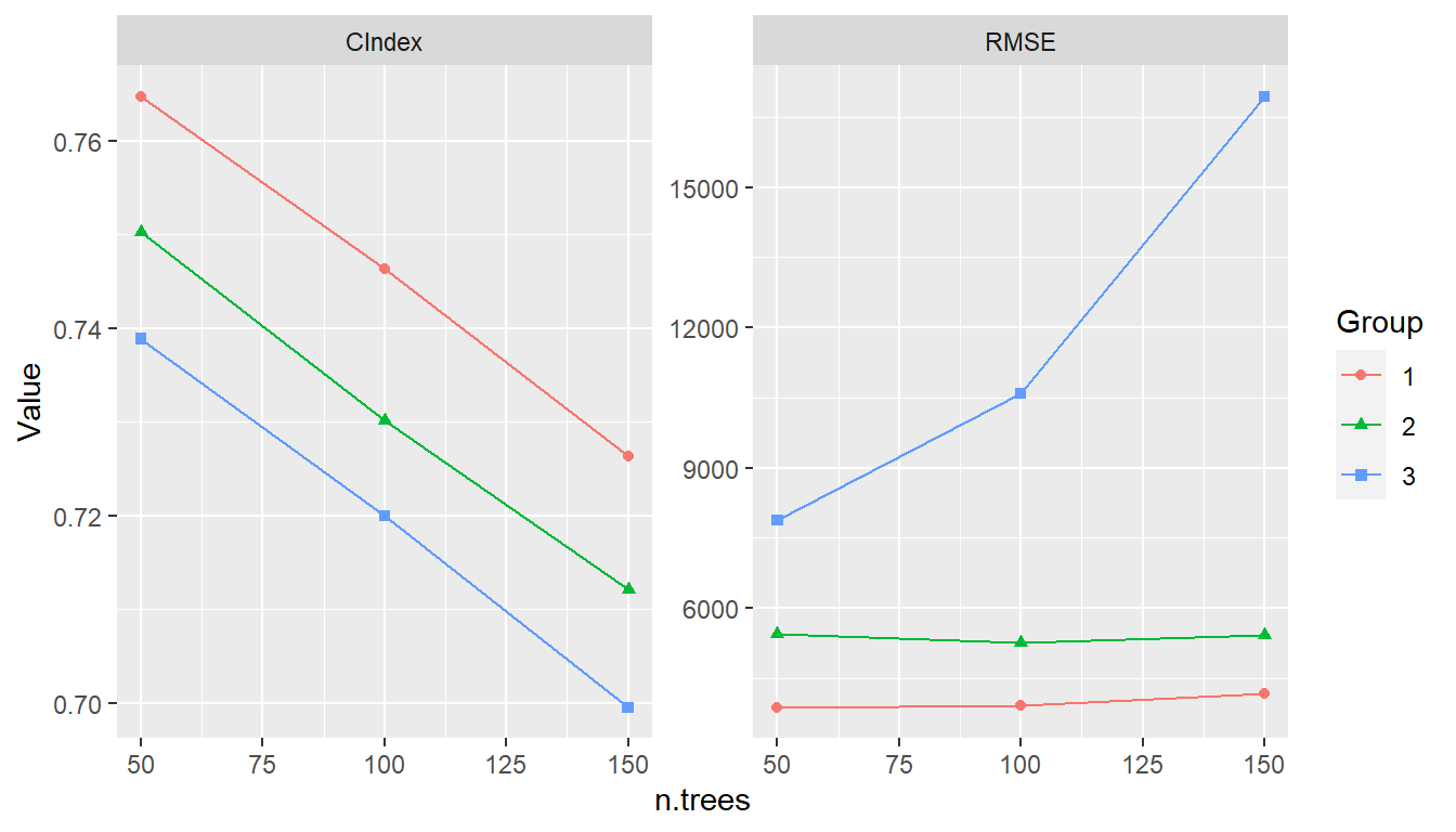
Model Selection
Model selection can be conducted by calling fit()
with a SelectedModel
to automatically choose from any combination of models and model
parameters. Selection has as a special case the just-discussed tuning of
a single model over a grid of parameter values. Combinations of model
functions, function names, or objects can be supplied to SelectedModel()
in order to define sets of candidate models from which to select. An expand_model()
helper function is additionally available to expand a model over a grid
of tuning parameters for inclusion in the candidate set if so
desired.
## Model interface for model selection
sel_model <- SelectedModel(
  expand_model(GBMModel, n.trees = c(50, 100), interaction.depth = 1:2),
  GLMNetModel(lambda = 0.01),
  CoxModel,
  SurvRegModel
)

## Fit the selected model
fit(surv_fo, data = surv_train, model = sel_model)
Selection may also be performed over candidate sets that include
tuned models. For instance, the SelectedModel()
function is applicable to sets containing different classes of models
each individually tuned over a grid of parameters.
## Model interface for selection among tuned models
sel_tun_model <- SelectedModel(
  TunedModel(GBMModel, control = surv_means_control),
  TunedModel(GLMNetModel, control = surv_means_control),
  TunedModel(CoxModel, control = surv_means_control)
)

## Fit the selected tuned model
fit(surv_fo, data = surv_train, model = sel_tun_model)
Ensemble Learning
Ensemble learning models combine \(m = 1, \ldots, M\) base models as a strategy to improve predictive performance. Two methods implemented in MachineShop are stacked regression (Breiman 1996) and super learners (van der Laan et al. 2007). Stacked regression fits a linear combination of predictions from specified base learners to produce a prediction function of the form \[ \hat{f}(x) = \sum_{m=1}^M \hat{w}_m \hat{f}_m(x). \] Stacking weights \(w\) are estimated by (constrained) least squares regression of case responses \(y_i\) on predictions \(\hat{f}_m^{-\kappa(i)}(x_i)\) from learners fit to data subsamples \(-\kappa(i)\) not containing the corresponding cases. In particular, they are obtained as the solution \[ \hat{w} = \underset{w}{\operatorname{argmin}} \sum_{i=1}^{N}\left(y_i - \sum_{m=1}^{M} w_m \hat{f}_m^{-\kappa(i)}(x_i) \right)^2 \] subject to the constraints that all \(w_m \ge 0\) and \(\sum_m w_m = 1\). K-fold cross-validation is the default subsampling method employed in the estimation, with the other resampling methods provided by the package available as options. Survival outcomes are handled with a modified version of the stacked regression algorithm in which
- minimization of least squares is replaced by maximization of Harrell’s concordance index (1982) to accommodate censoring, and
- prediction can only be performed on the same response type used for the model fit; i.e., either survival means or survival probabilities at given follow-up times.
Super learners are a generalization of stacked regression that fit a
specified model, such as GBMModel,
to case responses \(y_i\), base learner
predictions \(\hat{f}_m^{-\kappa(i)}(x_i)\), and
optionally also to the original predictor variables \(x_i\). Given below are examples of a
stacked regression and super learner each fit with gradient boosted,
random forest, and Cox regression base learners. A separate gradient
boosted model is used as the super learner in the latter.
## Stacked regression
stackedmodel <- StackedModel(CoxModel, CForestModel, GLMBoostModel)
res_stacked <- resample(surv_fo, data = surv_train, model = stackedmodel)
summary(res_stacked)
#>          Statistic
#> Metric         Mean   Median        SD       Min       Max NA
#>   C-Index 0.7294869 0.762963 0.1275484 0.5194805 0.8556701  0

## Super learner
supermodel <- SuperModel(CoxModel, CForestModel, GLMBoostModel,
                         model = GBMModel)
res_super <- resample(surv_fo, data = surv_train, model = supermodel)
summary(res_super)
#>          Statistic
#> Metric         Mean    Median        SD       Min       Max NA
#>   C-Index 0.7534803 0.8325472 0.1243104 0.5748899 0.8454545  0
Methodology
Combinations and multiple levels of nested meta-functions, inputs,
and models are possible. If model fitting involves a single
meta-function, performances of the inputs or models under consideration
are estimated with standard resampling, and the best performing model is
returned. Nestings of meta-functions are trained with nested resampling.
Consider the example below in which training involves input tuning and
model selection. In particular, a preprocessing recipe is tuned over the
number of predictor-derived principal components and model selection is
of an untuned GBMModel,
a tuned GBMModel,
and a StackedModel.
## Preprocessing recipe with PCA steps
pca_rec <- recipe(y ~ ., data = surv_train) %>%
  role_case(stratum = y) %>%
  step_center(all_predictors()) %>%
  step_scale(all_predictors()) %>%
  step_pca(all_predictors(), id = "PCA")

## Tuning grid of number of PCA components
pca_grid <- expand_steps(
  PCA = list(num_comp = 1:3)
)

## Input specification
tun_rec <- TunedInput(pca_rec, grid = pca_grid)

## Model specification
sel_model <- SelectedModel(
  GBMModel,
  TunedModel(GBMModel),
  StackedModel(CoxModel, TunedModel(CForestModel), TunedModel(GBMModel))
)

## Model fit and final trained model
model_fit <- fit(tun_rec, model = sel_model)
as.MLModel(model_fit)
Model fitting proceeds with instances of the specified model
selection nested within each of the input tuning grid parameter values.
Tuning of GBMModel
and construction of StackedModel
are further nested within the model selection, with tuning of CForestModel
and GBMModel
nested within StackedModel.
Altogether, there are four levels of meta-input and meta-model functions
in the hierarchy.
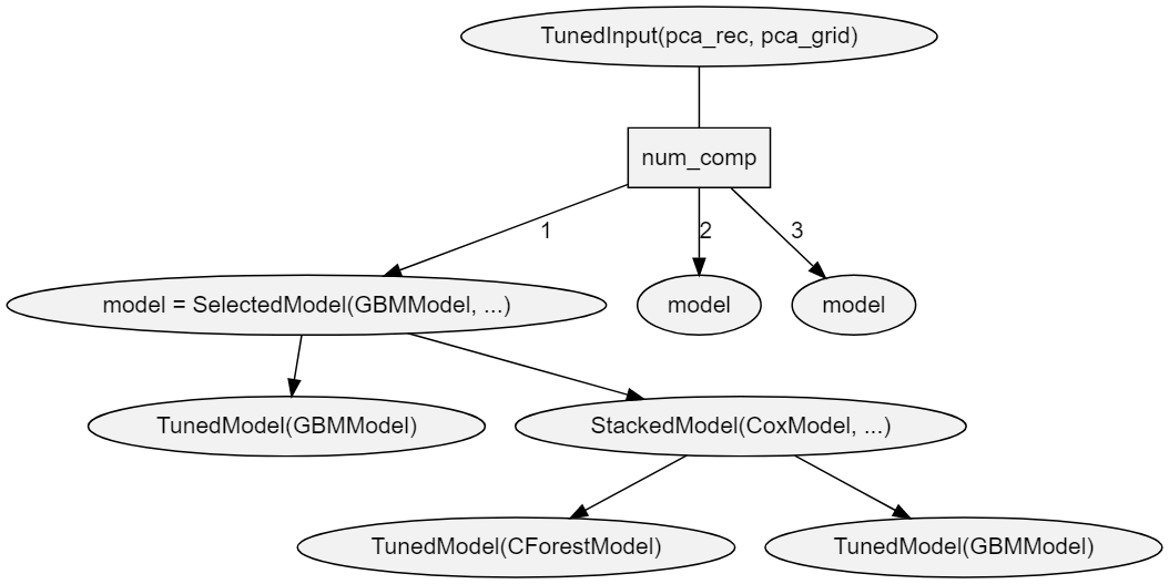
Each meta-function is fit based on resample estimation (default: cross-validation) of predictive performance. When one meta-function is nested within another, nested resampling is employed, as illustrated in the figure below.
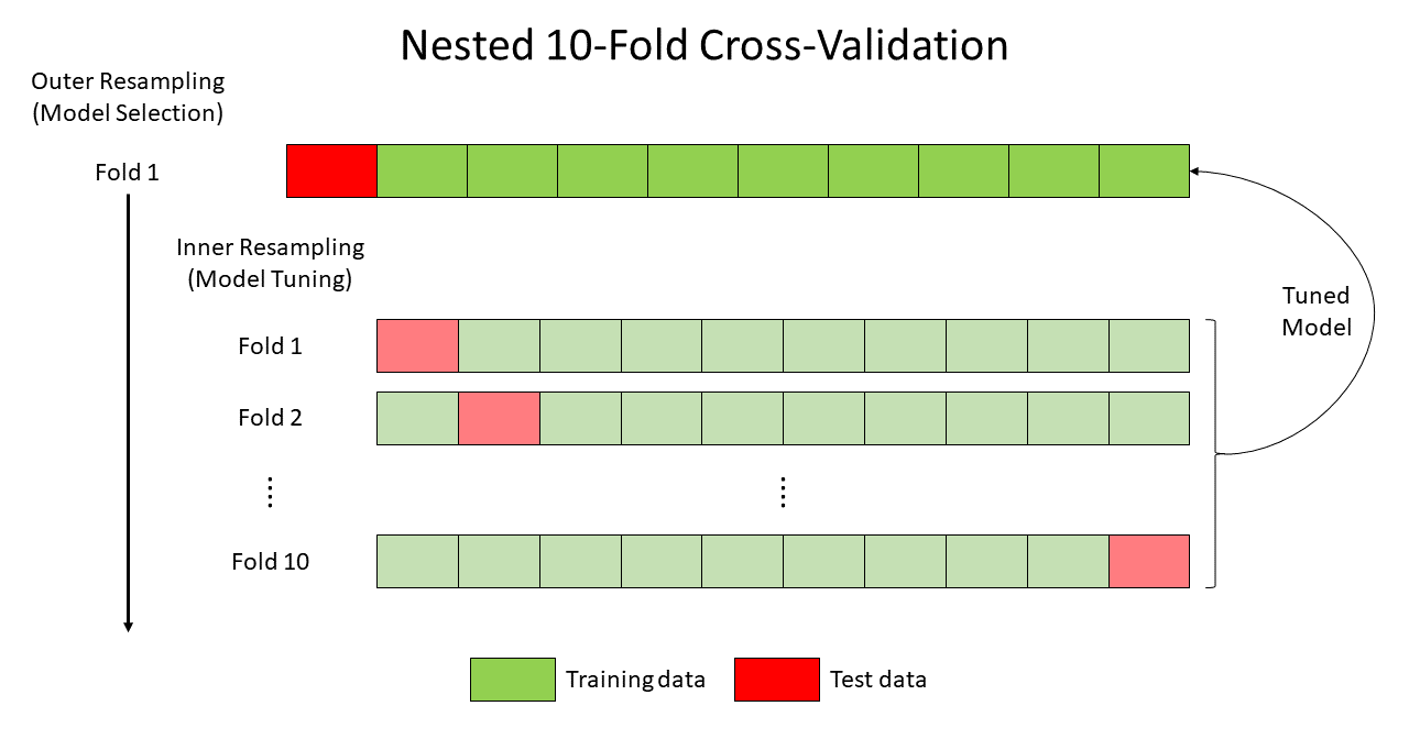
Nesting of resampling routines is repeated recursively when a fit
involves multiple levels of nested meta-functions. For example,
predictive performance estimation for the training of TunedInput(pca_rec, grid = pca_grid)
involves up to three nested meta functions: SelectedModel(...)
→ StackedModel(...)
→ TunedModel(CForestModel).
For this relationship, an outer and three nested inner resampling loops
are executed as follows. First, CForestModel
is tuned at the third inner resampling loop. Second, the tuned model is
passed to the second inner loop for construction of StackedModel.
Third, the constructed model is passed to the first inner loop for model
selection from the candidate set. Finally, the selected model is passed
to the outer loop for tuning of the preprocessing recipe. Based on
resample performance estimation of the entire input/model specification,
one principal component is selected for the GBMModel.
#> === $TrainingStep1 ==========================================================
#> === TrainingStep object ===
#>
#> Optimization method: Grid Search
#> TunedModelRecipe log:
#> # A tibble: 3 × 4
#>   name          selected params$PCA$num_comp metrics$`C-Index`
#>   <chr>         <lgl>                  <int>             <dbl>
#> 1 ModelRecipe.1 TRUE                       1             0.741
#> 2 ModelRecipe.2 FALSE                      2             0.733
#> 3 ModelRecipe.3 FALSE                      3             0.691
#>
#> Selected row: 1
#> Metric: C-Index = 0.7405534
In order to identify and return a final model fitted to the entire
input data, the hierarchy is traversed from top to bottom along the path
determined by the choice at each node. Steps along the path are labeled
TrainStep1 and TrainStep2 in the output. As
seen above in TrainStep1, one principal component is first
selected for the tuned input. Using an input recipe with one principal
component, the entire dataset is refit at TrainStep2 to
finally select GBMModel.
#> === $TrainingStep2 ==========================================================
#> === TrainingStep object ===
#>
#> Optimization method: Grid Search
#> SelectedModel log:
#> # A tibble: 3 × 4
#>   name         selected params$id  metrics$`C-Index`
#>   <chr>        <lgl>    <chr>                  <dbl>
#> 1 GBMModel     TRUE     model.1mQk             0.740
#> 2 TunedModel   FALSE    model.hRF5             0.735
#> 3 StackedModel FALSE    model.CYj0             0.653
#>
#> Selected row: 1
#> Metric: C-Index = 0.7399641
After the series of training steps reaches the bottom of its hierarchy, the final model is fitted to the entire dataset and returned.
#> --- MLModel object ----------------------------------------------------------
#>
#> Model name: GBMModel
#> Label: Trained Generalized Boosted Regression
#> Package: gbm
#> Response types: factor, numeric, PoissonVariate, Surv
#> Case weights support: TRUE
#> Missing case removal: response
#> Tuning grid: TRUE
#> Variable importance: TRUE
#>
#> Parameters:
#> List of 5
#>  $ n.trees          : num 100
#>  $ interaction.depth: num 1
#>  $ n.minobsinnode   : num 10
#>  $ shrinkage        : num 0.1
#>  $ bag.fraction     : num 0.5
Generalization performance of the entire process can be estimated
with a call to resample().
## Generalization performance of the modeling strategy
resample(tun_rec, model = sel_model)
There is no conceptual limit to the number of nested inputs and models that can be specified with the package. However, there are some practical issues to consider.
- Computational Expense
- Computational expense of nested resampling increases exponentially. For instance, execution of r levels of a nested 10-fold cross-validation algorithm is an O(10r) operation. Runtimes can be decreased by registering multiple cores to run the resampling algorithms in parallel. However, the exponential increase in computational complexity quickly outpaces the number of available cores.
- Data Reduction
- Training data is reduced at each subsequent resampling level. For 10-fold cross-validation and a training set of N total cases, there will be 0.9r cases available at each fold of the rth resampling algorithm. Bootstrapping could be used, as an alternative to cross-validation, to ensure N cases at each resampling level. However, the number of unique cases at level r will be decreased to approximately N(2/3)r.
ModelSpecification Class
The ModelSpecification
class allows response and predictor variables and a model that defines
the relationship between them to be packaged together into a single
container for ease of model fitting and assessment. The inputs and
models described previously can be included in a ModelSpecification.
Resampling control and a method for optimizing tuning parameters are
also part of the specification. A ModelSpecification
object with its default or a user-specified control method has the
following characteristics.
- Tuning of input and model objects is performed simultaneously over a global grid of their parameter values.
- The specification’s control method overrides those of any included
TunedInputorTunedModel. ModeledInput,SelectedInput, andSelectedModelobjects are not allowed in the specification.
The default tuning parameter optimization method is an exhaustive
grid search. Other methods can be employed with the set_optim
functions.
| Optimization Function | Method |
|---|---|
set_optim_bayes() |
Bayesian optimization with a Gaussian process model (Snoek et al. 2012) |
set_optim_bfgs() |
Limited-memory modification of quasi-Newton BFGS optimization (Byrd et al. 1995) |
set_optim_grid() |
Exhaustive or random grid search |
set_optim_method() |
User-defined optimization function |
set_optim_pso() |
Particle swarm optimization (Bratton and Kennedy 2007) |
set_optim_sann() |
Simulated annealing (Belisle 1992) |
## Preprocessing recipe with PCA steps
pca_rec <- recipe(y ~ ., data = surv_train) %>%
  role_case(stratum = y) %>%
  step_center(all_predictors()) %>%
  step_scale(all_predictors()) %>%
  step_pca(all_predictors(), id = "PCA")

## Tuning grid of number of PCA components
pca_grid <- expand_steps(
  PCA = list(num_comp = 1:3)
)

## Model specification
(modelspec <- ModelSpecification(
  TunedInput(pca_rec, grid = pca_grid),
  TunedModel(GBMModel),
  control = surv_means_control
))
#> --- ModelSpecification object -----------------------------------------------
#>
#> === ModelRecipe object ===
#>
#> ID: input.HoL8
#> Outcome: y
#> Predictors: sex, age, year, thickness, ulcer
#> Untrained step IDs: step_center = center_4KNaz, step_scale = scale_CuYFW,
#>   step_pca = PCA
#> Number of observations: 136
#>
#> === MLModel object ===
#>
#> Model name: GBMModel
#> Label: Generalized Boosted Regression
#> ID: model.bshV
#>
#> === Grid ===
#>
#> # A tibble: 27 × 2
#>    input.HoL8$PCA$num_comp model.bshV$n.trees $interaction.depth
#>                      <int>              <int>              <int>
#>  1                       1                 50                  1
#>  2                       1                 50                  2
#>  3                       1                 50                  3
#>  4                       1                100                  1
#>  5                       1                100                  2
#>  6                       1                100                  3
#>  7                       1                150                  1
#>  8                       1                150                  2
#>  9                       1                150                  3
#> 10                       2                 50                  1
#> # ℹ 17 more rows
#>
#> === TrainingParams object ===
#>
#> ... GridSearch object
#> Label: Grid Search
#>
#> ... CVControl object
#> Label: K-Fold Cross-Validation
#> Folds: 5
#> Repeats: 3

## Model fit with Bayesian optimization
bayes_fit <- modelspec %>% set_optim_bayes %>% fit
as.MLModel(bayes_fit)
#> --- MLModel object ----------------------------------------------------------
#>
#> Model name: GBMModel
#> Label: Trained Generalized Boosted Regression
#> Package: gbm
#> Response types: factor, numeric, PoissonVariate, Surv
#> Case weights support: TRUE
#> Missing case removal: response
#> Tuning grid: TRUE
#> Variable importance: TRUE
#>
#> Parameters:
#> List of 5
#>  $ n.trees          : num 50
#>  $ interaction.depth: num 1
#>  $ n.minobsinnode   : num 10
#>  $ shrinkage        : num 0.1
#>  $ bag.fraction     : num 0.5
#>
#> === $TrainingStep1 ==========================================================
#> === TrainingStep object ===
#>
#> Optimization method: Bayesian Optimization
#> ModelSpecification log:
#> # A tibble: 15 × 5
#>    name         epoch selected params$input.HoL8$PCA$num_comp metrics$`C-Index`
#>    <chr>        <int> <lgl>                             <dbl>             <dbl>
#>  1 ModelSpec.1      0 FALSE                                 2             0.714
#>  2 ModelSpec.2      0 FALSE                                 3             0.745
#>  3 ModelSpec.3      0 FALSE                                 3             0.740
#>  4 ModelSpec.4      0 FALSE                                 2             0.727
#>  5 ModelSpec.5      0 FALSE                                 1             0.723
#>  6 ModelSpec.6      1 TRUE                                  3             0.755
#>  7 ModelSpec.7      2 FALSE                                 1             0.744
#>  8 ModelSpec.8      3 FALSE                                 3             0.755
#>  9 ModelSpec.9      4 FALSE                                 3             0.754
#> 10 ModelSpec.10     5 FALSE                                 3             0.747
#> # ℹ 5 more rows
#> # ℹ 1 more variable: params$model.bshV <tibble[,2]>
#>
#> Selected row: 6
#> Metric: C-Index = 0.7549613
Alternatively, a value of NULL may be specified as the
control method in a ModelSpecifiction
so that any package input or model object is allowed, object-specific
control structures and training parameters are used for selection and
tuning, and objects are trained sequentially with nested resampling
rather than simultaneously with a global grid. This, in essence, is how
input and model objects are handled if passed separately in to the fit()
and resample()
functions apart from a ModelSpecification.
Having them together in a ModelSpecifiction
has the advantage of simplifying the function calls to be in terms of
one object instead of two.
ModelSpecification(
  TunedInput(pca_rec, grid = pca_grid),
  TunedModel(GBMModel),
  control = NULL
)
#> --- ModelSpecification object -----------------------------------------------
#>
#> === TunedModelRecipe object ===
#>
#> Outcome: y
#> Predictors: sex, age, year, thickness, ulcer
#> Untrained steps: step_center, step_scale, step_pca
#> Number of observations: 136
#>
#> === TunedModel object ===
#>
#> Model name: TunedModel
#> Label: Grid Tuned GBMModel
#>
#> ... MLModel object
#> Model name: GBMModel
#> Label: Generalized Boosted Regression
Global Settings
Core default behaviors of functions in the package can be viewed or
changed globally through the settings()
function. The function accepts one or more character names of settings
to view, name = value pairs giving the values of settings
to change, or a vector of these, with available settings summarized
below.
control-
function, function name, or object defining a default resampling method
[default:
"CVControl"]. cutoff- numeric (0, 1) threshold above which binary factor probabilities are classified as events and below which survival probabilities are classified [default: 0.5].
distr.SurvMeans-
character string specifying distributional approximations to estimated
survival curves for predicting survival means. Choices are
"empirical"for the Kaplan-Meier estimator,"exponential","rayleigh", or"weibull"(default). distr.SurvProbs-
character string specifying distributional approximations to estimated
survival curves for predicting survival events/probabilities. Choices
are
"empirical"(default) for the Kaplan-Meier estimator,"exponential","rayleigh", or"weibull". grid-
sizeargument toTuningGrid()indicating the number of parameter-specific values to generate automatically for tuning of models that have pre-defined grids or aTuningGrid()function, function name, or object [default: 3]. method.EmpiricalSurv-
character string specifying the empirical method of estimating baseline
survival curves for Cox proportional hazards-based models. Choices are
"breslow"or"efron"(default). metrics.ConfusionMatrix-
function, function name, or vector of these with which to calculate
performance metrics for confusion matrices [default:
c(Accuracy = "accuracy", Kappa = "kappa2", `Weighted Kappa` = "weighted_kappa2", Sensitivity = "sensitivity", Specificity = "specificity")]. metrics.factor-
function, function name, or vector of these with which to calculate
performance metrics for factor responses [default:
c(Brier = "brier", Accuracy = "accuracy", Kappa = "kappa2", `Weighted Kappa` = "weighted_kappa2", `ROC AUC` = "roc_auc", Sensitivity = "sensitivity", Specificity = "specificity")]. metrics.matrix-
function, function name, or vector of these with which to calculate
performance metrics for matrix responses [default:
c(RMSE = "rmse", R2 = "r2", MAE = "mae")]. metrics.numeric-
function, function name, or vector of these with which to calculate
performance metrics for numeric responses [default:
c(RMSE = "rmse", R2 = "r2", MAE = "mae")]. metrics.Surv-
function, function name, or vector of these with which to calculate
performance metrics for survival responses [default:
c(`C-Index` = "cindex", Brier = "brier", `ROC AUC` = "roc_auc", Accuracy = "accuracy")]. print_max-
number of models or data rows to show with print methods or
Infto show all [default: 10]. require-
names of installed packages to load during parallel execution of
resampling algorithms [default:
"MachineShop"]. reset- character names of settings to reset to their default values.
RHS.formula- non-modifiable character vector of operators and functions allowed in traditional formula specifications.
stat.Curve-
function or character string naming a function to compute one summary
statistic at each cutoff value of resampled metrics in performance
curves, or
NULLfor resample-specific metrics [default:"base::mean"]. stat.Resample-
function or character string naming a function to compute one summary
statistic to control the ordering of models in plots [default:
"base::mean"]. stat.TrainingParams-
function or character string naming a function to compute one summary
statistic on resampled performance metrics for input selection or tuning
or for model selection or tuning [default:
"base::mean"]. stats.PartialDependence-
function, function name, or vector of these with which to compute
partial dependence summary statistics [default:
c(Mean = "base::mean")]. stats.Resample-
function, function name, or vector of these with which to compute
summary statistics on resampled performance metrics [default:
c(Mean = "base::mean", Median = "stats::median", SD = "stats::sd", Min = "base::min", Max = "base::max")].
A call to settings()
with "reset" will restore all package defaults and with no
arguments will display the current values of all. Settings may also be
supplied as a single unnamed argument which is a named list. Partial
matching of setting names is supported. The setting value is returned if
only one is specified to view. Otherwise, a list is returned with the
values of specified settings as they existed prior to any requested
changes. Such a list can be passed as an argument to settings()
to restore their values.
## Change settings
presets <- settings(control = "BootControl", grid = 10)

## View one setting
settings("control")
#> [1] "BootControl"

## View multiple settings
settings("control", "grid")
#> $control
#> [1] "BootControl"
#>
#> $grid
#> --- TuningGrid object -------------------------------------------------------
#>
#> Grid size: 10
#> Random samples: FALSE

## Restore the previous settings
settings(presets)
Package Extensions
Custom models and metrics can be defined with MLModel()
and MLMetric()
for use with the model fitting, prediction, and performance assessment
tools provided by the package.
Custom Models
The MLModel()
function creates a model object that can be used with the previously
described fitting functions. It take the following arguments.
name- character name of the object to which the model is assigned.
label-
optional character descriptor for the model (default:
name). packages-
character vector of packages upon which the model depends. Each name may
be optionally followed by a comment in parentheses specifying a version
requirement. The comment should contain a comparison operator,
whitespace and a valid version number,
e.g.
"xgboost (>= 1.3.0)". response_types-
character vector of response variable types to which the model can be
fit. Supported types are
"binary","BinomialVariate","DiscreteVariate","factor","matrix","NegBinomialVariate","numeric","ordered","PoissonVariate", and"Surv". fit-
model fitting function whose arguments are a
formula, aModelFramenameddata, caseweights, and an ellipsis. Argumentdatamay be converted to a data frame with theas.data.frame()function as is commonly needed. The fit function should return the object resulting from the model fit. predict-
prediction function whose arguments are the
objectreturned byfit(), aModelFramenamednewdataof predictor variables, optional vector oftimesat which to predict survival, and an ellipsis. Argumentdatamay be converted to a data frame with theas.data.frame()function as needed. Values returned by the function should be formatted according to the response variable types below.
factor: matrix whose columns contain the probabilities for multi-level factors or vector of probabilities for the second level of binary factors.matrix: matrix of predicted responses.numeric: vector or column matrix of predicted responses.Surv: matrix whose columns contain survival probabilities attimesif supplied or vector of predicted survival means otherwise.
varimp-
optional variable importance function whose arguments are the
objectreturned byfit(), optional arguments passed from calls tovarimp(), and an ellipsis. The function should return a vector of importance values named after the predictor variables or a matrix or data frame whose rows are named after the predictors.
## Logistic regression model extension
LogisticModel <- MLModel(
  name = "LogisticModel",
  label = "Logistic Model",
  response_types = "binary",
  weights = TRUE,
  fit = function(formula, data, weights, ...) {
    glm(formula, data = as.data.frame(data), weights = weights,
        family = binomial, ...)
  },
  predict = function(object, newdata, ...) {
    predict(object, newdata = as.data.frame(newdata), type = "response")
  },
  varimp = function(object, ...) {
    pchisq(coef(object)^2 / diag(vcov(object)), 1)
  }
)
Custom Metrics
The MLMetric()
function creates a metric object that can be used as previously
described for the model performance metrics. Its first argument is a
function to compute the metric, defined to accept observed
and predicted as the first two arguments and with an
ellipsis to accommodate others. Its remaining arguments are as
follows.
name- character name of the object to which the metric is assigned.
label-
optional character descriptor for the metric (default:
name). maximize- logical indicating whether higher values of the metric correspond to better predictive performance.
## F2 score metric extension
f2_score <- MLMetric(
  function(observed, predicted, ...) {
    f_score(observed, predicted, beta = 2, ...)
  },
  name = "f2_score",
  label = "F2 Score",
  maximize = TRUE
)
Usage
Once created, model and metric extensions can be used with the package-supplied fitting and performance functions.
## Logistic regression analysis
data(Pima.tr, package = "MASS")
res <- resample(type ~ ., data = Pima.tr, model = LogisticModel)
summary(performance(res, metric = f2_score))
#>           Statistic
#> Metric          Mean    Median         SD       Min       Max NA
#>   f2_score 0.5499676 0.5714286 0.05093445 0.4761905 0.6060606  0