Example

Diabetes in Pima Indian Women

Characteristics of Pima Indian women tested for diabetes are used in this example to predict their disease statuses.

Characteristic	Value
Number of women	392
diabetes
pos	130 (33.16%)
neg	262 (66.84%)
pregnant
Median (Range)	2 (0, 17)
glucose
Median (Range)	119 (56, 198)
pressure
Median (Range)	70 (24, 110)
triceps
Median (Range)	29 (7, 63)
insulin
Median (Range)	125.5 (14, 846)
mass
Median (Range)	33.2 (18.2, 67.1)
pedigree
Median (Range)	0.4495 (0.085, 2.420)
age
Median (Range)	27 (21, 81)

Training Set Analysis

## Analysis libraries
library(MachineShop)
library(ggplot2)

## Parallel processing
library(doParallel)
registerDoParallel(cores = 6)

## Dataset
data(PimaIndiansDiabetes2, package = "mlbench")
Pima <- na.omit(PimaIndiansDiabetes2)

## Model formula
fo <- diabetes ~ .

## Model selected from tuned models
selected_model <- SelectedModel(TunedModel(KNNModel, grid = 5),
                                TunedModel(NNetModel, grid = 5),
                                TunedModel(RandomForestModel, grid = 5))

## Model fit
model_fit <- fit(fo, data = Pima, model = selected_model)

## Variable importance
vi <- varimp(model_fit)
plot(vi)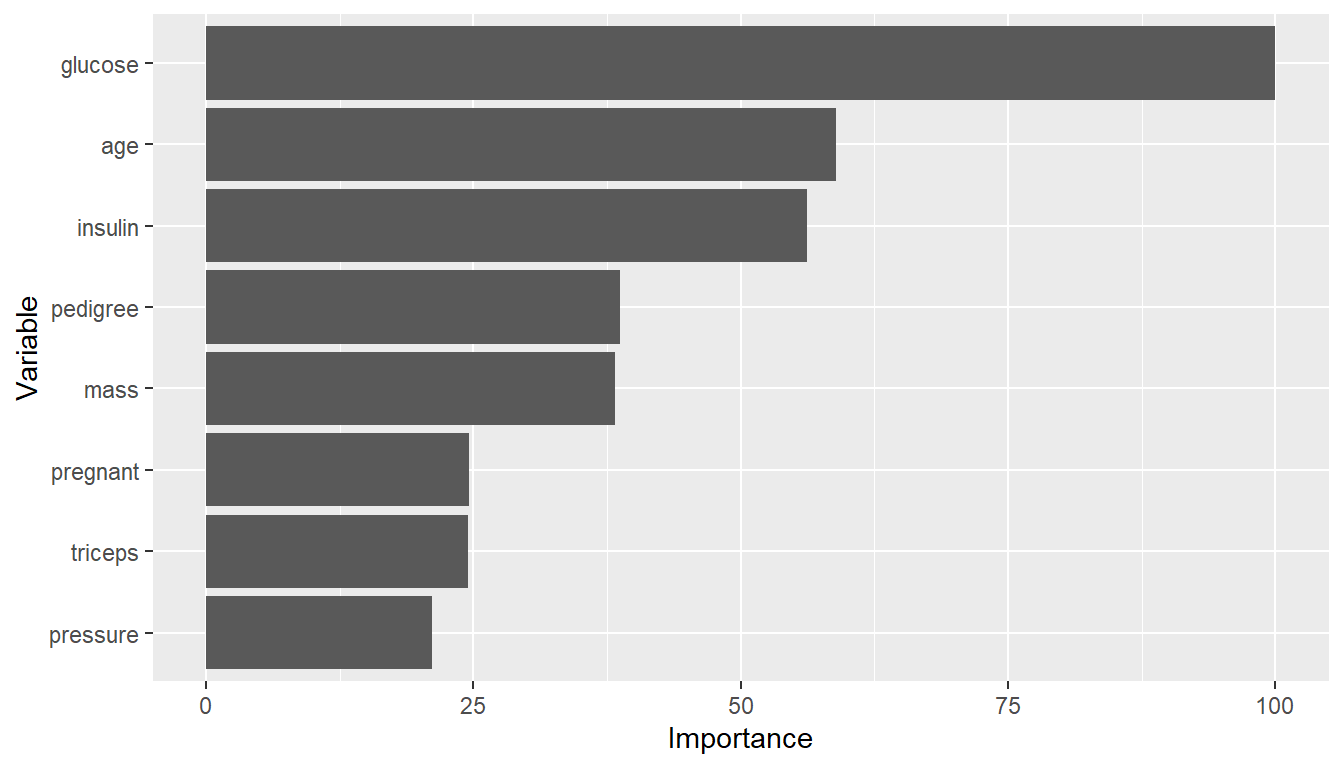

Generalization Performance

## Resample estimation with cross-validation
res <- resample(fo, data = Pima, model = selected_model, control = CVControl)

## Estimated performance
summary(performance(res))
#>              Statistic
#> Metric             Mean    Median         SD       Min       Max NA
#>   Brier       0.1441490 0.1385509 0.04313255 0.1060426 0.2562013  0
#>   Accuracy    0.7857051 0.7974359 0.06529521 0.6410256 0.8717949  0
#>   Kappa       0.4999248 0.5123220 0.15928724 0.1250000 0.6808511  0
#>   ROC AUC     0.8531339 0.8786982 0.08404156 0.6375740 0.9186391  0
#>   Sensitivity 0.6153846 0.6153846 0.13074409 0.3076923 0.7692308  0
#>   Specificity 0.8700855 0.8682336 0.06074830 0.8076923 1.0000000  0

## Variable probability cutoff
summary(performance(res, cutoff = 0.25))
#>              Statistic
#> Metric             Mean    Median         SD       Min       Max NA
#>   Brier       0.1441490 0.1385509 0.04313255 0.1060426 0.2562013  0
#>   Accuracy    0.7499359 0.7435897 0.06878381 0.6410256 0.8500000  0
#>   Kappa       0.5013070 0.5080645 0.14027061 0.2500000 0.6946565  0
#>   ROC AUC     0.8531339 0.8786982 0.08404156 0.6375740 0.9186391  0
#>   Sensitivity 0.8846154 0.9230769 0.12162606 0.6153846 1.0000000  0
#>   Specificity 0.6831909 0.6730769 0.06161579 0.5925926 0.7777778  0

ROC Curve

## True positive and false positive rates over all probability cutoffs
roc <- performance_curve(res)

## ROC curve
plot(roc, diagonal = TRUE) + coord_fixed()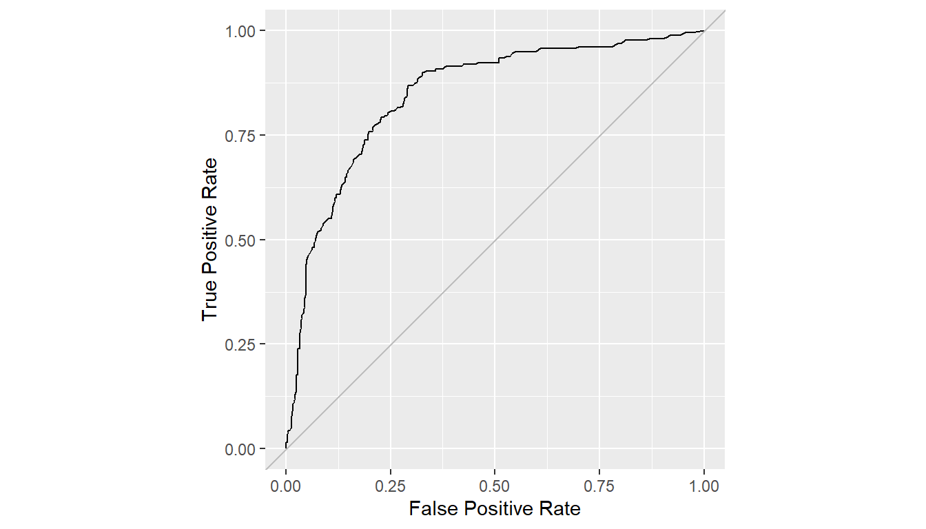

## Area under the curve
auc(roc)
#> Model: SelectedModel
#> [1] 0.8464381

Confusion Matrices

(conf <- confusion(res))
#> --- ConfusionList object ----------------------------------------------------------------------
#> 
#> === $SelectedModel ============================================================================
#> === BinaryConfusionMatrix object ===
#>          Observed
#> Predicted neg pos
#>       neg 228  50
#>       pos  34  80

summary(conf)
#> --- $SelectedModel ----------------------------------------------------------------------------
#> Number of responses: 392
#> Accuracy (SE): 0.7857143 (0.02072459)
#> Majority class: 0.6683673
#> Kappa: 0.5011514
#> 
#>                   neg       pos
#> Observed    0.6683673 0.3316327
#> Predicted   0.7091837 0.2908163
#> Agreement   0.5816327 0.2040816
#> Sensitivity 0.8702290 0.6153846
#> Specificity 0.6153846 0.8702290
#> PPV         0.8201439 0.7017544
#> NPV         0.7017544 0.8201439

plot(conf)
#> $SelectedModel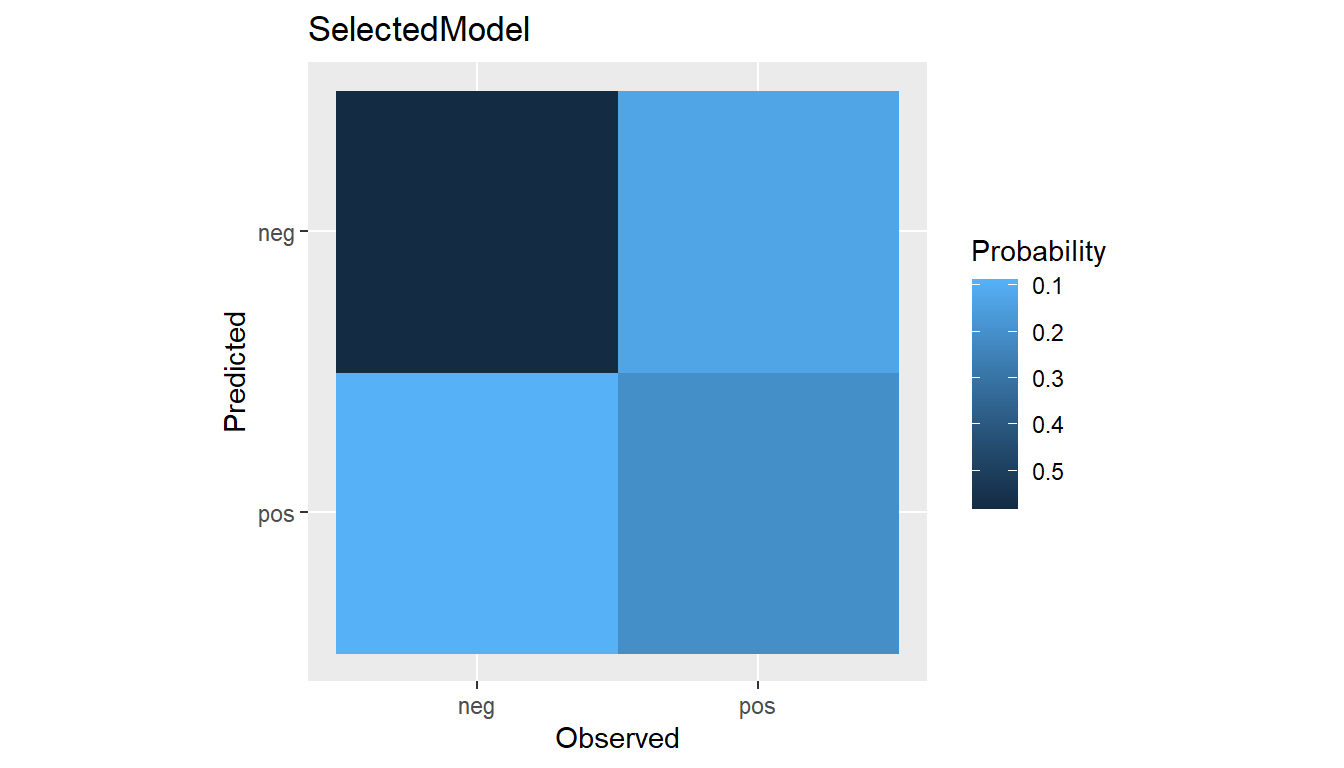

## Variable probability cutoff
summary(confusion(res, cutoff = 0.25))
#> --- $SelectedModel ----------------------------------------------------------------------------
#> Number of responses: 392
#> Accuracy (SE): 0.75 (0.02187044)
#> Majority class: 0.6683673
#> Kappa: 0.5017122
#> 
#>                   neg       pos
#> Observed    0.6683673 0.3316327
#> Predicted   0.4948980 0.5051020
#> Agreement   0.4566327 0.2933673
#> Sensitivity 0.6832061 0.8846154
#> Specificity 0.8846154 0.6832061
#> PPV         0.9226804 0.5808081
#> NPV         0.5808081 0.9226804

Calibration Curve

cal <- calibration(res, breaks = NULL)
plot(cal, se = TRUE)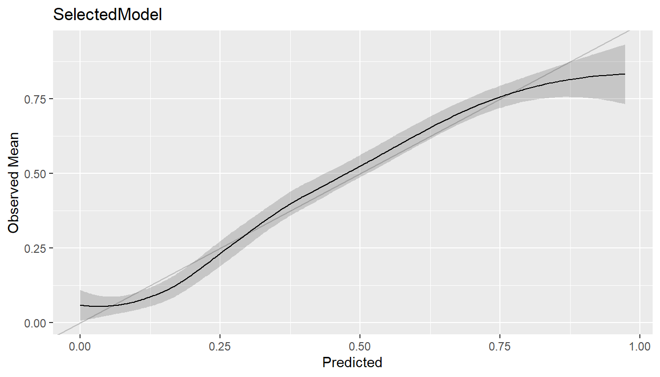

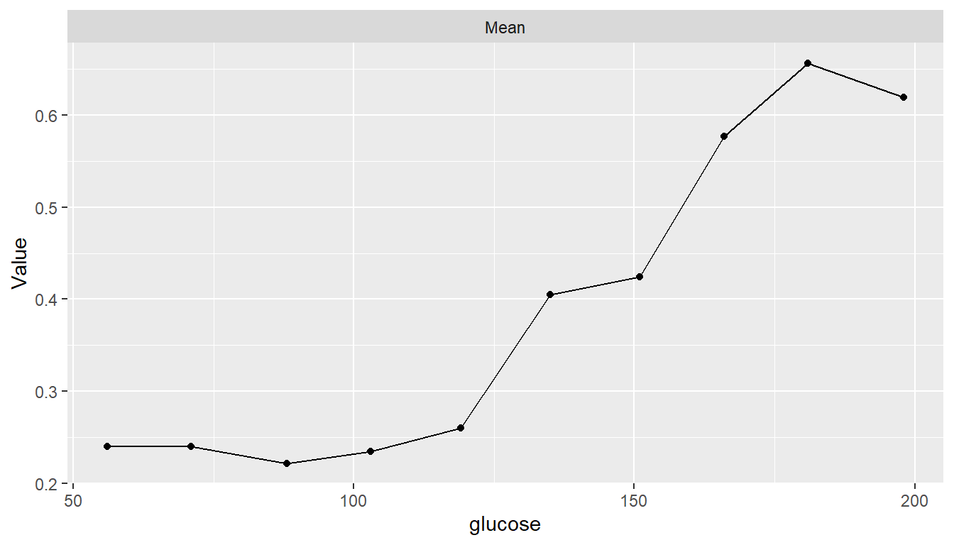
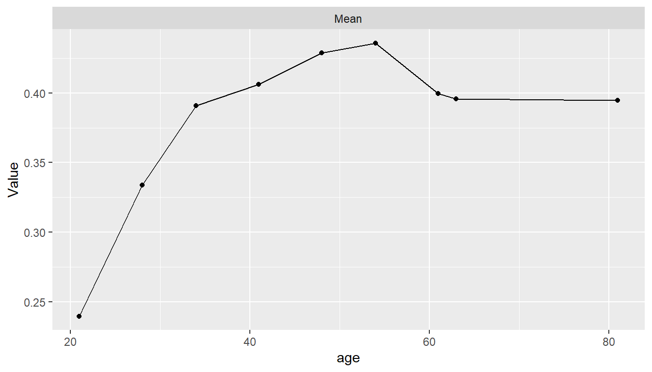
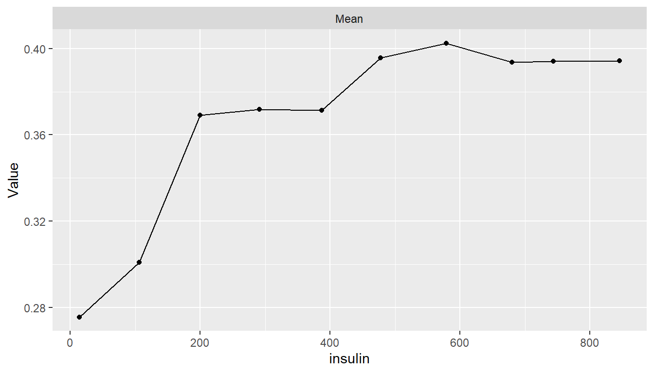
Partial Dependence Plots

pd <- dependence(model_fit, select = c(glucose, age, insulin))
plot(pd)