Example
IC Home Prices
In this example, a generalized boosted model is developed to predict the prices of homes sold in Iowa City, IA during 2005-2008.
| Characteristic | Value |
|---|---|
| Number of homes | 753 |
| sale_amount | |
| Median (Range) | $158,000 ($38,250, $815,000) |
| sale_year | |
| Median (Range) | 2006 (2005, 2008) |
| sale_month | |
| Median (Range) | 6 (1, 12) |
| built | |
| Median (Range) | 1979 (1873, 2007) |
| style | |
| Home | 515 (68.39%) |
| Condo | 238 (31.61%) |
| construction | |
| 1 1/2 Story Frame | 25 (3.32%) |
| 1 Story Brick | 24 (3.19%) |
| 1 Story Condo | 45 (5.98%) |
| 1 Story Frame | 336 (44.62%) |
| 2 Story Brick | 10 (1.33%) |
| 2 Story Condo | 27 (3.59%) |
| 2 Story Frame | 180 (23.9%) |
| Split Foyer Frame | 76 (10.09%) |
| Split Level Frame | 30 (3.98%) |
| base_size (sq ft) | |
| Median (Range) | 933 (240, 3440) |
| garage1_size (sq ft) | |
| Median (Range) | 0 (0, 1065) |
| garage2_size (sq ft) | |
| Median (Range) | 0 (0, 856) |
| lot_size (sq ft) | |
| Median (Range) | 7592 (137, 158123) |
| bedrooms | |
| 1-2 | 249 (33.07%) |
| 3 | 280 (37.18%) |
| 4 | 168 (22.31%) |
| 5+ | 56 (7.44%) |
| basement | |
| Yes | 578 (76.76%) |
| No | 175 (23.24%) |
| ac | |
| Yes | 679 (90.17%) |
| No | 74 (9.83%) |
| attic | |
| Yes | 53 (7.04%) |
| No | 700 (92.96%) |
| lon | |
| Median (Range) | -91.5158 (-91.60575, -91.46307) |
| lat | |
| Median (Range) | 41.65263 (41.62804, 41.69092) |
Training Set Analysis
## Analysis libraries
library(MachineShop)
library(ggplot2)

## Training and test sets
set.seed(123)
train_indices <- sample(nrow(ICHomes), nrow(ICHomes) * 2 / 3)
trainset <- ICHomes[train_indices, ]
testset <- ICHomes[-train_indices, ]

## Model formula
fo <- sale_amount ~ .

## Boosted regression model tuned with the training set
model_fit <- TunedModel(GBMModel, grid = 5) %>% fit(fo, data = trainset)

## Variable importance
vi <- varimp(model_fit)
plot(vi)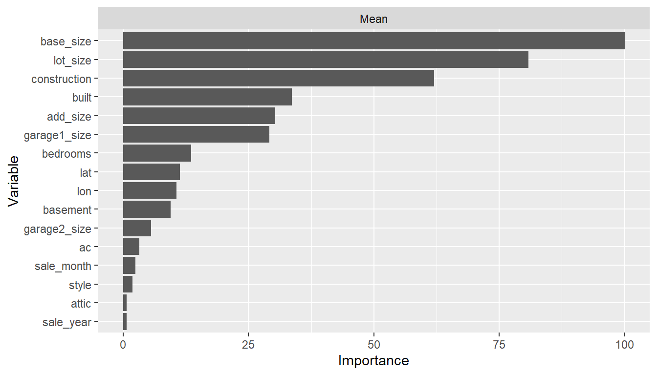
## Performance plotted over the grid points
(tuned_model <- as.MLModel(model_fit))
#> --- MLModel object ----------------------------------------------------------
#>
#> Model name: GBMModel
#> Label: Trained Generalized Boosted Regression
#> Package: gbm
#> Response types: factor, numeric, PoissonVariate, Surv
#> Case weights support: TRUE
#> Missing case removal: response
#> Tuning grid: TRUE
#> Variable importance: TRUE
#>
#> Parameters:
#> List of 5
#>  $ n.trees          : int 250
#>  $ interaction.depth: int 4
#>  $ n.minobsinnode   : num 10
#>  $ shrinkage        : num 0.1
#>  $ bag.fraction     : num 0.5
#>
#> === $TrainingStep1 ==========================================================
#> === TrainingStep object ===
#>
#> Optimization method: Grid Search
#> TunedModel log:
#> # A tibble: 25 × 4
#>    name        selected params$n.trees $interaction.depth metrics$RMSE   $R2
#>    <chr>       <lgl>             <int>              <int>        <dbl> <dbl>
#>  1 GBMModel.1  FALSE                50                  1       56750. 0.592
#>  2 GBMModel.2  FALSE                50                  2       53242. 0.641
#>  3 GBMModel.3  FALSE                50                  3       51911. 0.659
#>  4 GBMModel.4  FALSE                50                  4       50832. 0.672
#>  5 GBMModel.5  FALSE                50                  5       50068. 0.685
#>  6 GBMModel.6  FALSE               100                  1       52998. 0.636
#>  7 GBMModel.7  FALSE               100                  2       50227. 0.677
#>  8 GBMModel.8  FALSE               100                  3       49925. 0.679
#>  9 GBMModel.9  FALSE               100                  4       49399. 0.691
#> 10 GBMModel.10 FALSE               100                  5       49226. 0.692
#> # ℹ 15 more rows
#> # ℹ 1 more variable: metrics$MAE <dbl>
#>
#> Selected row: 24
#> Metric: RMSE = 48572.58
plot(tuned_model, type = "line")
#> $TrainingStep1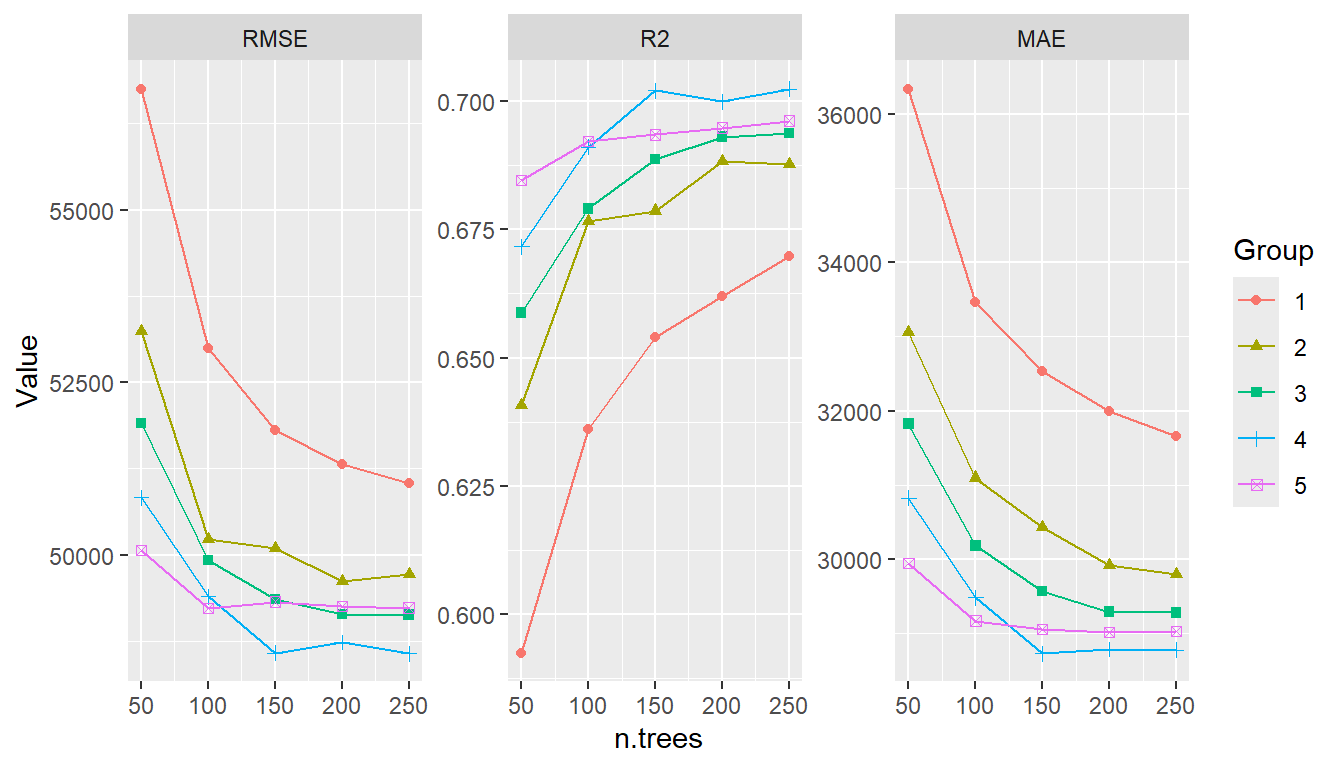
Generalization Performance
## Test set observed and predicted sale amounts
obs <- response(model_fit, newdata = testset)
pred <- predict(model_fit, newdata = testset)

## Test set performance
performance(obs, pred)
#>         RMSE           R2          MAE
#> 4.435582e+04 7.292781e-01 2.642282e+04
Calibration Curve
cal <- calibration(obs, pred, breaks = NULL)
plot(cal, se = TRUE)
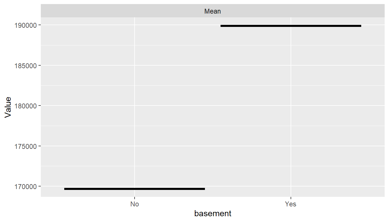
Partial Dependence Plots
## Marginal predictor effects
pd <- dependence(model_fit, select = c(base_size, built, basement))
plot(pd)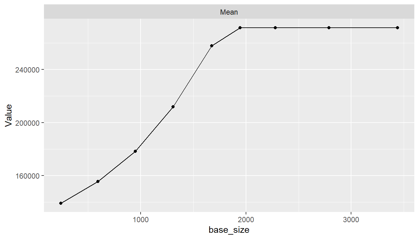

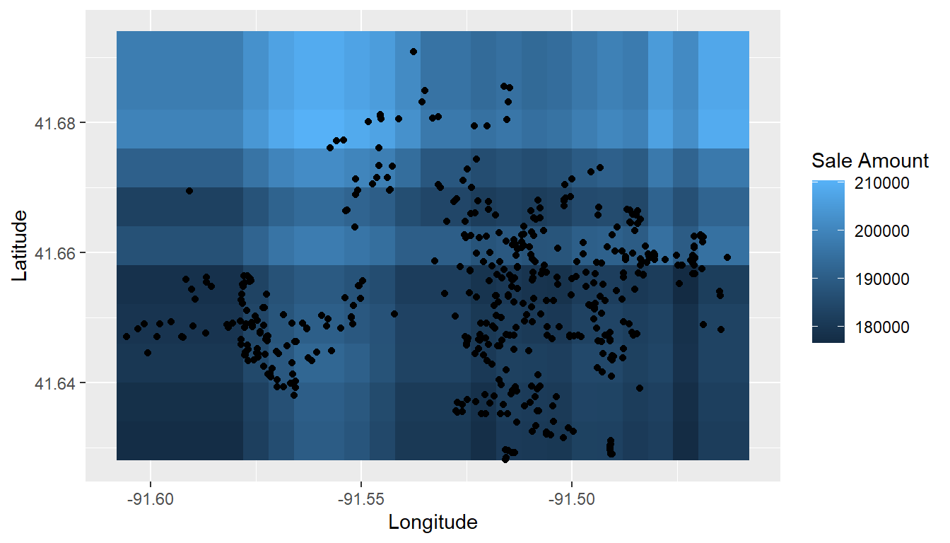
## Spatial distribution
pd <- dependence(model_fit, select = c(lon, lat), interaction = TRUE, n = 25)
df <- cbind(pd$Predictors, sale_amount = pd$Value)
ggplot(df) +
  stat_summary_2d(aes(lon, lat, z = sale_amount), binwidth = 0.006) +
  geom_point(aes(lon, lat), data = trainset) +
  labs(x = "Longitude", y = "Latitude", fill = "Sale Amount")