Example
Iris Flowers Species
The following illustrates use of the package to predict the species of flowers in Edgar Anderson’s iris data set.
| Characteristic | Value |
|---|---|
| Number of flowers | 150 |
| Species | |
| setosa | 50 (33.33%) |
| versicolor | 50 (33.33%) |
| virginica | 50 (33.33%) |
| Sepal.Length | |
| Median (Range) | 5.8 (4.3, 7.9) |
| Sepal.Width | |
| Median (Range) | 3 (2.0, 4.4) |
| Petal.Length | |
| Median (Range) | 4.35 (1.0, 6.9) |
| Petal.Width | |
| Median (Range) | 1.3 (0.1, 2.5) |
Training and Test Set Analysis
## Analysis libraries
library(MachineShop)
library(magrittr)

## Training and test sets
set.seed(123)
train_indices <- sample(nrow(iris), nrow(iris) * 2 / 3)
trainset <- iris[train_indices, ]
testset <- iris[-train_indices, ]

## Model formula
fo <- Species ~ .

## Models available for factor responses
modelinfo(factor(0)) %>% names
#>  [1] "AdaBagModel"       "AdaBoostModel"     "BARTModel"
#>  [4] "C50Model"          "CForestModel"      "EarthModel"
#>  [7] "FDAModel"          "GBMModel"          "GLMModel"
#> [10] "GLMNetModel"       "KNNModel"          "LDAModel"
#> [13] "LMModel"           "MDAModel"          "NaiveBayesModel"
#> [16] "NNetModel"         "ParsnipModel"      "PDAModel"
#> [19] "PLSModel"          "QDAModel"          "RandomForestModel"
#> [22] "RangerModel"       "RFSRCModel"        "RPartModel"
#> [25] "SelectedModel"     "StackedModel"      "SuperModel"
#> [28] "SVMModel"          "SVMANOVAModel"     "SVMBesselModel"
#> [31] "SVMLaplaceModel"   "SVMLinearModel"    "SVMPolyModel"
#> [34] "SVMRadialModel"    "SVMSplineModel"    "SVMTanhModel"
#> [37] "TreeModel"         "TunedModel"        "XGBModel"
#> [40] "XGBDARTModel"      "XGBLinearModel"    "XGBTreeModel"

## Model-specific information
modelinfo(GBMModel)
#> $GBMModel
#> $GBMModel$label
#> [1] "Generalized Boosted Regression"
#>
#> $GBMModel$packages
#> [1] "gbm"
#>
#> $GBMModel$response_types
#> [1] "factor"         "numeric"        "PoissonVariate" "Surv"
#>
#> $GBMModel$weights
#> [1] TRUE
#>
#> $GBMModel$na.rm
#> [1] "response"
#>
#> $GBMModel$arguments
#> function (distribution = character(), n.trees = 100, interaction.depth = 1,
#>     n.minobsinnode = 10, shrinkage = 0.1, bag.fraction = 0.5)
#> NULL
#>
#> $GBMModel$grid
#> [1] TRUE
#>
#> $GBMModel$varimp
#> [1] TRUE

## Generalized boosted model fit to training set
iris_fit <- fit(fo, data = trainset, model = GBMModel)

## Variable importance
(vi <- varimp(iris_fit))
#> --- VariableImportance object -----------------------------------------------
#> Method: permute
#> Metric: brier
#> Scale: 0.009790379
#> Values:
#>                     Mean
#> Petal.Length 100.0000000
#> Petal.Width   42.4880573
#> Sepal.Length   4.4254716
#> Sepal.Width    0.4421709

plot(vi)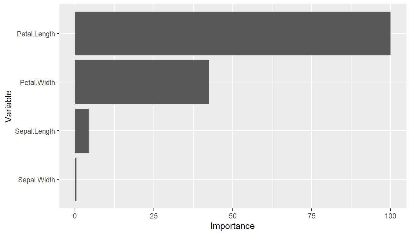
## Test set predicted probabilities
predict(iris_fit, newdata = testset, type = "prob") %>% head
#>         setosa   versicolor    virginica
#> [1,] 0.9999203 7.962238e-05 1.019789e-07
#> [2,] 0.9999804 1.917579e-05 3.924656e-07
#> [3,] 0.9999804 1.917579e-05 3.924656e-07
#> [4,] 0.9999736 2.615002e-05 2.758932e-07
#> [5,] 0.9999015 9.838405e-05 1.019770e-07
#> [6,] 0.9998846 1.153391e-04 1.019753e-07

## Test set predicted classifications
predict(iris_fit, newdata = testset) %>% head
#> [1] setosa setosa setosa setosa setosa setosa
#> Levels: setosa versicolor virginica

## Test set performance
obs <- response(iris_fit, newdata = testset)
pred <- predict(iris_fit, newdata = testset, type = "prob")
performance(obs, pred)
#>      Brier   Accuracy      Kappa    ROC AUC
#> 0.07933867 0.96000000 0.93939394 0.99511600
Resampling
## Resample estimation of model performance
(res <- resample(fo, data = iris, model = GBMModel, control = CVControl))
#> --- Resample object ---------------------------------------------------------
#>
#> Model: GBMModel
#> Sampling variables:
#> # A tibble: 150 × 2
#>    Case  Stratification$`(strata)`
#>    <chr> <fct>
#>  1 1     setosa
#>  2 2     setosa
#>  3 3     setosa
#>  4 4     setosa
#>  5 5     setosa
#>  6 6     setosa
#>  7 7     setosa
#>  8 8     setosa
#>  9 9     setosa
#> 10 10    setosa
#> # ℹ 140 more rows
#>
#> === CVControl object ===
#>
#> Label: K-Fold Cross-Validation
#> Folds: 10
#> Repeats: 1

summary(res)
#>           Statistic
#> Metric          Mean    Median         SD          Min       Max NA
#>   Brier    0.0948393 0.1177027 0.07251105 8.113202e-05 0.2178928  0
#>   Accuracy 0.9466667 0.9333333 0.04216370 8.666667e-01 1.0000000  0
#>   Kappa    0.9200000 0.9000000 0.06324555 8.000000e-01 1.0000000  0
#>   ROC AUC  0.9786667 1.0000000 0.02961481 9.333333e-01 1.0000000  0

plot(res)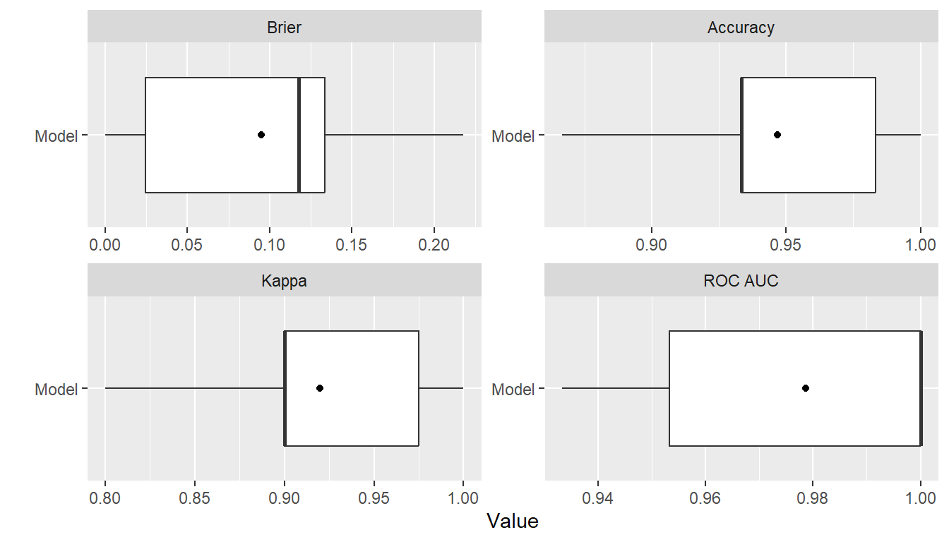
Performance Metrics
## Default performance metrics
performance(res) %>% summary
#>           Statistic
#> Metric          Mean    Median         SD          Min       Max NA
#>   Brier    0.0948393 0.1177027 0.07251105 8.113202e-05 0.2178928  0
#>   Accuracy 0.9466667 0.9333333 0.04216370 8.666667e-01 1.0000000  0
#>   Kappa    0.9200000 0.9000000 0.06324555 8.000000e-01 1.0000000  0
#>   ROC AUC  0.9786667 1.0000000 0.02961481 9.333333e-01 1.0000000  0

## Metrics available for the resample output
metricinfo(res) %>% names
#> [1] "accuracy"      "auc"           "brier"         "cross_entropy"
#> [5] "kappa2"        "pr_auc"        "roc_auc"

## User-specified metrics
performance(res, c(accuracy, kappa2)) %>% summary
#>           Statistic
#> Metric          Mean    Median         SD       Min Max NA
#>   accuracy 0.9466667 0.9333333 0.04216370 0.8666667   1  0
#>   kappa2   0.9200000 0.9000000 0.06324555 0.8000000   1  0
Model Tuning
## Tune over a grid of model parameters
iris_fit <- TunedModel(
  GBMModel,
  grid = expand_params(n.trees = c(25, 50, 100),
                       interaction.depth = 1:3,
                       n.minobsinnode = c(5, 10))
) %>% fit(fo, data = iris)

## Variable importance
varimp(iris_fit)
#> --- VariableImportance object -----------------------------------------------
#> Method: permute
#> Metric: brier
#> Scale: 0.008658078
#> Values:
#>                      Mean
#> Petal.Length 100.00000000
#> Petal.Width   24.47878599
#> Sepal.Width    0.11864159
#> Sepal.Length   0.07704569

## Plot performance over the grid points
tuned_model <- as.MLModel(iris_fit)
plot(tuned_model, type = "line")
#> $TrainingStep1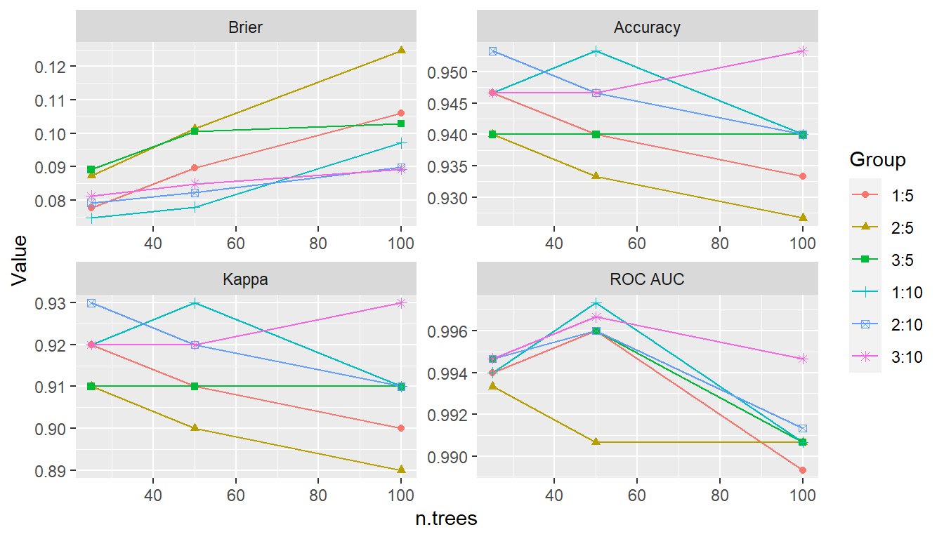
Model Comparisons
## Model comparisons
control <- CVControl(folds = 10, repeats = 5)

res1 <- resample(fo, data = iris, model = GBMModel(n.tree = 50), control = control)
res2 <- resample(fo, data = iris, model = RandomForestModel(ntree = 50), control = control)
res3 <- resample(fo, data = iris, model = NNetModel(size = 5), control = control)

res <- c(GBM = res1, RF = res2, NNet = res3)
summary(res)
#> , , Metric = Brier
#>
#>       Statistic
#> Model        Mean     Median         SD          Min       Max NA
#>   GBM  0.08222226 0.07922268 0.08986729 5.358880e-05 0.4860763  0
#>   RF   0.06954880 0.05661333 0.07295257 3.733333e-04 0.4088533  0
#>   NNet 0.09861942 0.00889123 0.13707365 2.027928e-20 0.6666545  0
#>
#> , , Metric = Accuracy
#>
#>       Statistic
#> Model       Mean    Median         SD       Min Max NA
#>   GBM  0.9506667 0.9333333 0.05183263 0.7333333   1  0
#>   RF   0.9533333 0.9333333 0.05429407 0.7333333   1  0
#>   NNet 0.9386667 1.0000000 0.09508559 0.6000000   1  0
#>
#> , , Metric = Kappa
#>
#>       Statistic
#> Model   Mean Median         SD Min Max NA
#>   GBM  0.926    0.9 0.07774894 0.6   1  0
#>   RF   0.930    0.9 0.08144110 0.6   1  0
#>   NNet 0.906    1.0 0.15307728 0.4   1  0
#>
#> , , Metric = ROC AUC
#>
#>       Statistic
#> Model       Mean Median         SD       Min Max NA
#>   GBM  0.9894667      1 0.01919420 0.9333333   1  0
#>   RF   0.9932000      1 0.01624584 0.9333333   1  0
#>   NNet 0.9722000      1 0.04787365 0.8333333   1  0

plot(res)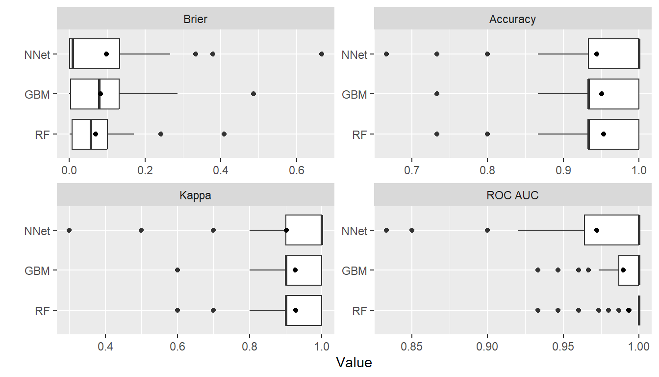
## Pairwise model differences and t-tests
perfdiff <- diff(res)
summary(perfdiff)
#> , , Metric = Brier
#>
#>             Statistic
#> Model               Mean        Median         SD         Min        Max NA
#>   GBM - RF    0.01267346  4.261331e-04 0.02768193 -0.02764053 0.07722295  0
#>   GBM - NNet -0.01639716 -7.783568e-05 0.10176021 -0.33292223 0.16154038  0
#>   RF - NNet  -0.02907062  3.669109e-04 0.10357991 -0.33226667 0.11246802  0
#>
#> , , Metric = Accuracy
#>
#>             Statistic
#> Model          Mean Median         SD         Min        Max NA
#>   GBM - RF   -0.004      0 0.02487155 -0.06666667 0.06666667  0
#>   GBM - NNet  0.008      0 0.07576069 -0.06666667 0.33333333  0
#>   RF - NNet   0.012      0 0.07338897 -0.06666667 0.33333333  0
#>
#> , , Metric = Kappa
#>
#>             Statistic
#> Model          Mean Median         SD  Min Max NA
#>   GBM - RF   -0.004      0 0.03475864 -0.1 0.1  0
#>   GBM - NNet  0.012      0 0.11890658 -0.1 0.5  0
#>   RF - NNet   0.016      0 0.11668902 -0.1 0.5  0
#>
#> , , Metric = ROC AUC
#>
#>             Statistic
#> Model                Mean Median         SD         Min        Max NA
#>   GBM - RF   -0.003733333      0 0.01152027 -0.04000000 0.01333333  0
#>   GBM - NNet  0.017266667      0 0.04738844 -0.05333333 0.16666667  0
#>   RF - NNet   0.021000000      0 0.04690053 -0.06666667 0.16666667  0

t.test(perfdiff)
#> --- PerformanceDiffTest object ----------------------------------------------
#>
#> Upper diagonal: mean differences (Model1 - Model2)
#> Lower diagonal: p-values
#> P-value adjustment method: holm
#>
#> , , Metric = Brier
#>
#>       Model2
#> Model1       GBM         RF        NNet
#>   GBM         NA 0.01267346 -0.01639716
#>   RF   0.6362196         NA -0.02907062
#>   NNet 0.8840076 0.88400758          NA
#>
#> , , Metric = Accuracy
#>
#>       Model2
#> Model1 GBM     RF  NNet
#>   GBM   NA -0.004 0.008
#>   RF     1     NA 0.012
#>   NNet   1  1.000    NA
#>
#> , , Metric = Kappa
#>
#>       Model2
#> Model1 GBM     RF  NNet
#>   GBM   NA -0.004 0.012
#>   RF     1     NA 0.016
#>   NNet   1  1.000    NA
#>
#> , , Metric = ROC AUC
#>
#>       Model2
#> Model1       GBM           RF       NNet
#>   GBM         NA -0.003733333 0.01726667
#>   RF   0.6664138           NA 0.02100000
#>   NNet 0.6664138  0.666413775         NA

plot(perfdiff)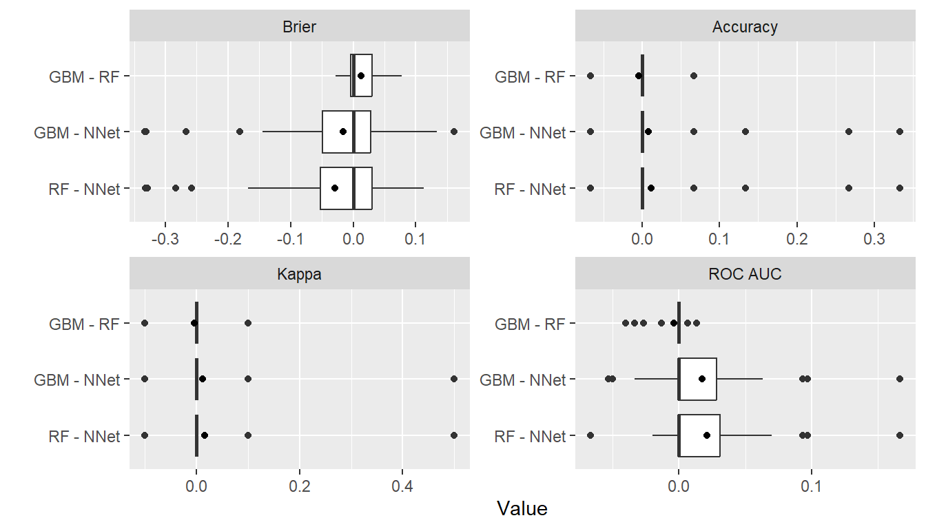
Ensemble Models
## Stacked regression
stackedmodel <- StackedModel(GBMModel, RandomForestModel, NNetModel)
res_stacked <- resample(fo, data = iris, model = stackedmodel)
summary(res_stacked)
#>           Statistic
#> Metric           Mean     Median         SD          Min       Max NA
#>   Brier    0.07818532 0.02915482 0.09773153 0.0006731487 0.3006319  0
#>   Accuracy 0.95333333 1.00000000 0.07062333 0.8000000000 1.0000000  0
#>   Kappa    0.93000000 1.00000000 0.10593499 0.7000000000 1.0000000  0
#>   ROC AUC  0.99333333 1.00000000 0.01133115 0.9733333333 1.0000000  0

## Super learner
supermodel <- SuperModel(GBMModel, RandomForestModel, NNetModel)
res_super <- resample(fo, data = iris, model = supermodel)
summary(res_super)
#>           Statistic
#> Metric           Mean    Median         SD          Min       Max NA
#>   Brier    0.09363295 0.0773554 0.08677424 1.272903e-06 0.2458399  0
#>   Accuracy 0.94666667 0.9666667 0.06885304 8.000000e-01 1.0000000  0
#>   Kappa    0.92000000 0.9500000 0.10327956 7.000000e-01 1.0000000  0
#>   ROC AUC  0.98800000 1.0000000 0.02126842 9.333333e-01 1.0000000  0
Calibration Curves
cal <- calibration(res1)
plot(cal, se = TRUE)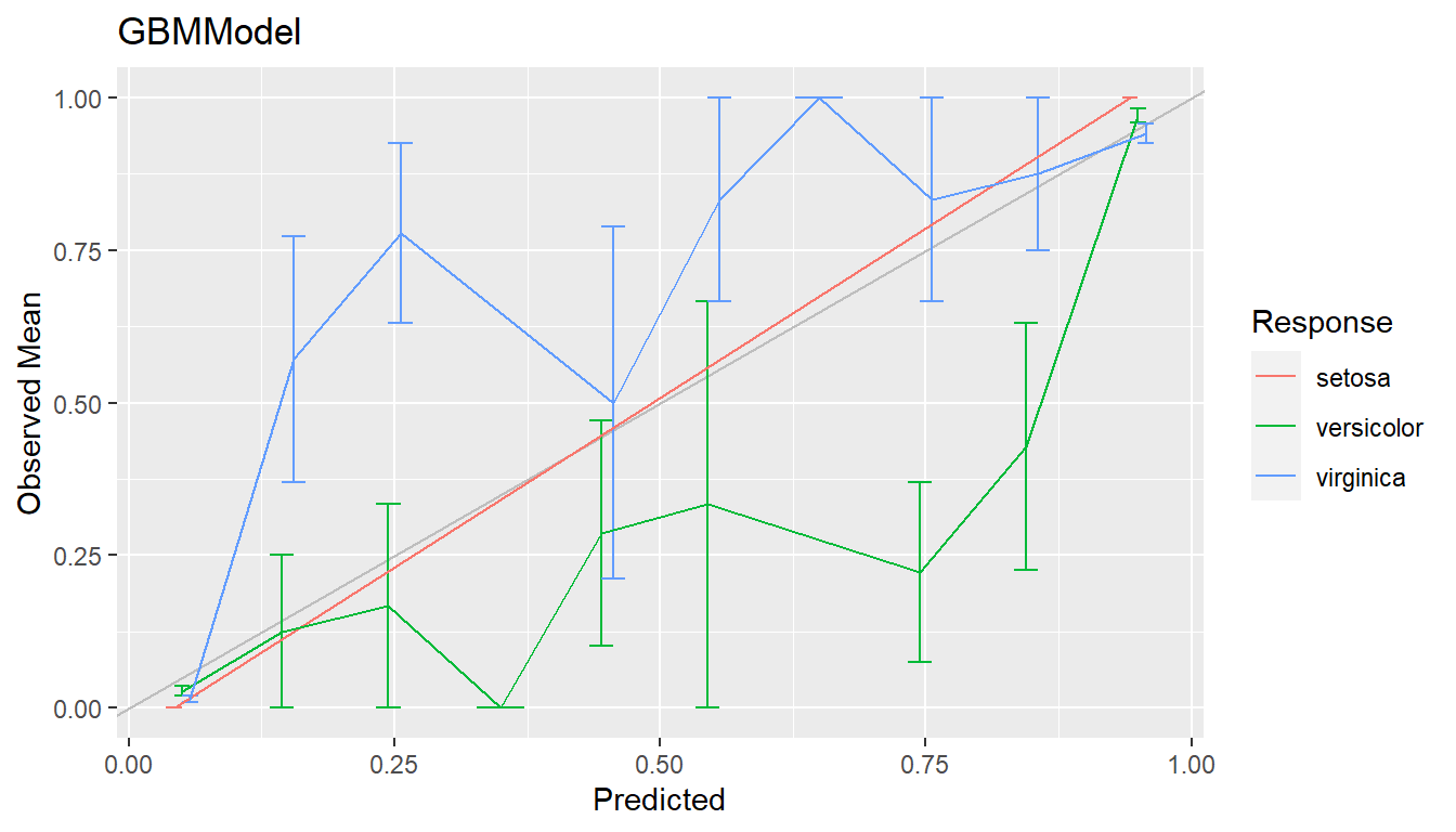
Confusion Matrices
(conf <- confusion(res1, cutoff = NULL))
#> --- ConfusionList object ----------------------------------------------------
#>
#> === $GBMModel ===============================================================
#> === ConfusionMatrix object ===
#>             Observed
#> Predicted          setosa   versicolor    virginica
#>   setosa     249.30932795   0.25221814   0.09391384
#>   versicolor   0.67430045 230.21683206  24.30257249
#>   virginica    0.01637160  19.53094980 225.60351367

summary(conf)
#> --- $GBMModel ---------------------------------------------------------------
#> Number of responses: 750
#> Accuracy (SE): 0.9401729 (0.008660086)
#> Majority class: 0.3333333
#> Kappa: 0.9102593
#>
#>                setosa versicolor virginica
#> Observed    0.3333333  0.3333333 0.3333333
#> Predicted   0.3328739  0.3402583 0.3268678
#> Agreement   0.3324124  0.3069558 0.3008047
#> Sensitivity 0.9972373  0.9208673 0.9024141
#> Specificity 0.9993077  0.9500463 0.9609054
#> PPV         0.9986136  0.9021258 0.9202641
#> NPV         0.9986196  0.9600184 0.9516757
plot(conf)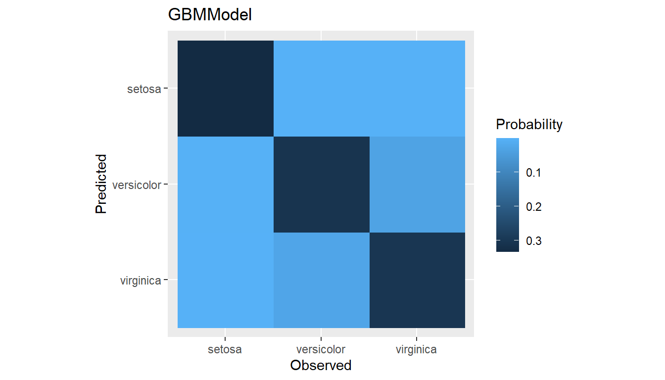
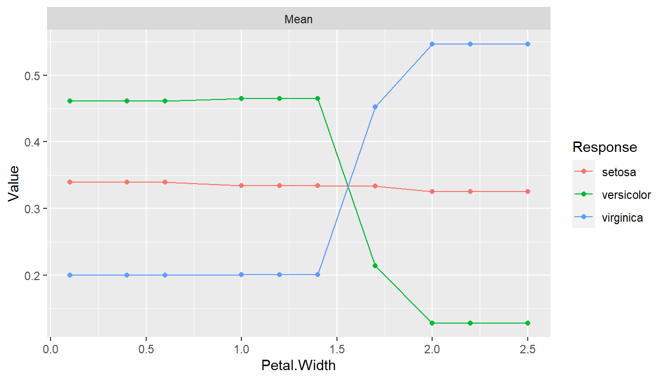
Partial Dependence Plots
pd <- dependence(iris_fit, select = c(Petal.Length, Petal.Width))
plot(pd)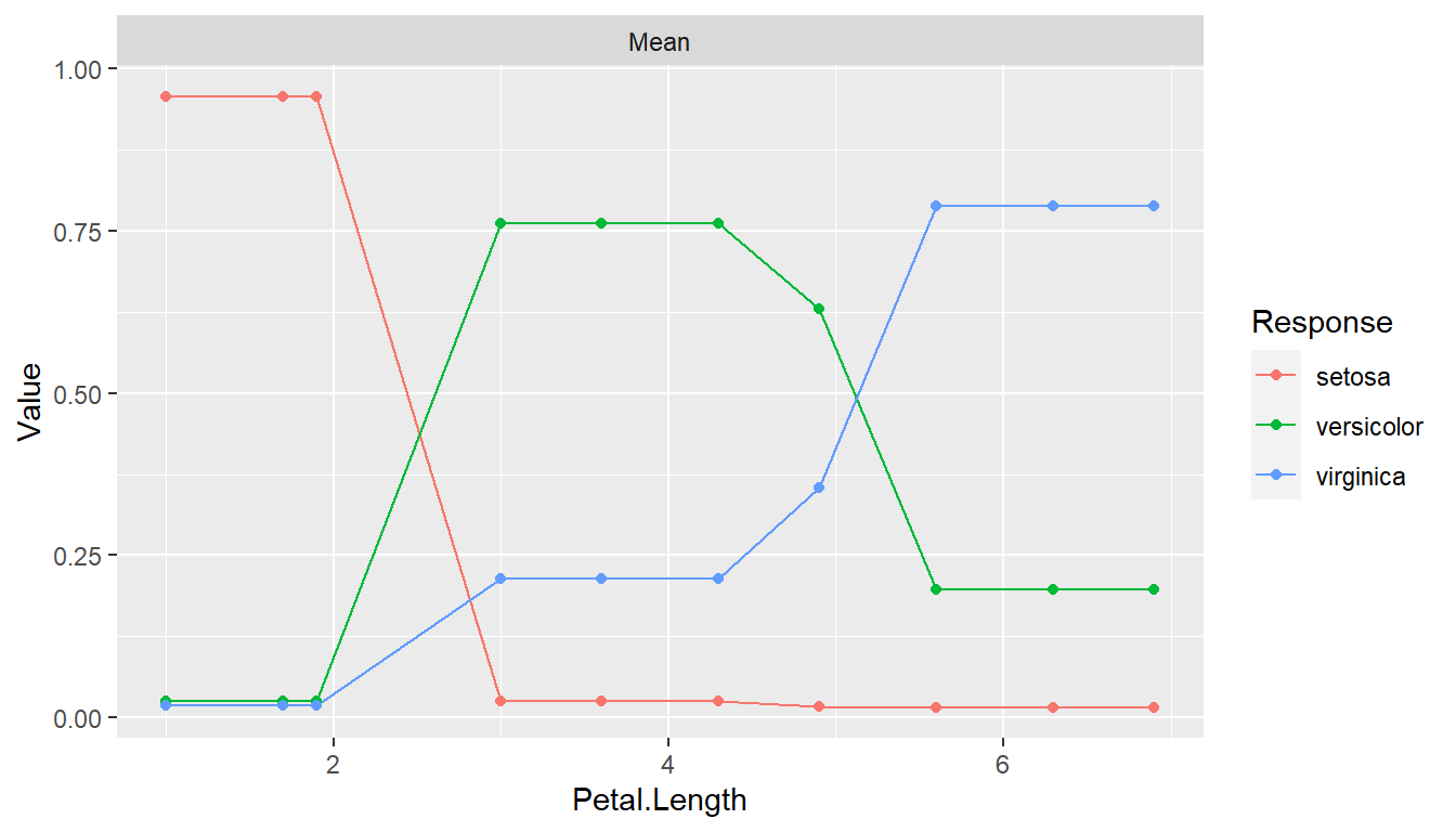
Preprocessing Recipe
library(recipes)

rec <- recipe(fo, data = iris) %>%
  role_case(stratum = Species)

iris_fit <- fit(rec, model = GBMModel)
varimp(iris_fit)
#> --- VariableImportance object -----------------------------------------------
#> Method: permute
#> Metric: brier
#> Scale: 0.0108775
#> Values:
#>                    Mean
#> Petal.Length 100.000000
#> Petal.Width   26.116233
#> Sepal.Width    3.552549
#> Sepal.Length   2.700857

res <- resample(rec, model = GBMModel, control = CVControl)
summary(res)
#>           Statistic
#> Metric          Mean     Median         SD          Min      Max NA
#>   Brier    0.1066633 0.08803549 0.13007118 2.811413e-05 0.407564  0
#>   Accuracy 0.9333333 0.93333333 0.08314794 7.333333e-01 1.000000  0
#>   Kappa    0.9000000 0.90000000 0.12472191 6.000000e-01 1.000000  0
#>   ROC AUC  0.9813333 1.00000000 0.02606734 9.333333e-01 1.000000  0