Using MRMCaov for R
Package Version 0.3.0
1 Introduction
A common study design for comparing the diagnostic performance of imaging modalities, or diagnostic tests, is to obtain modality-specific ratings from multiple readers of multiple cases (MRMC) whose true statuses are known. In such a design, receiver operating characteristic (ROC) indices, such as area under the ROC curve (ROC AUC), can be used to quantify correspondence between reader ratings and case status. Indices can then be compared statistically to determine if there are differences between modalities. However, special statistical methods are needed when readers or cases represent a random sample from a larger population of interest and there is overlap between modalities, readers, and/or cases. An ANOVA model designed for these characteristics of MRMC studies was initially proposed by Dorfman et al. (Dorfman, Berbaum, and Metz 1992) and Obuchowski and Rockette (Obuchowski and Rockette 1995) and later unified and improved by Hillis and colleagues (Hillis et al. 2005; Hillis 2007, 2018; Hillis, Berbaum, and Metz 2008). Their models are implemented in the MRMCaov R package (Brian J. Smith, Hillis, and Pesce 2022).
2 Obuchowski and Rockette Model
MRMCaov implements multi-reader multi-case analysis based on the Obuchowski and Rockette (1995) analysis of variance (ANOVA) model \[ \hat{\theta}_{ij} = \mu + \tau_i + R_j + (\tau R)_{ij} + \epsilon_{ij}, \] where \(i = 1,\ldots,t\) and \(j = 1,\ldots,r\) index diagnostic tests and readers; \(\hat{\theta}_{ij}\) is a reader performance metric, such as ROC AUC, estimated over multiple cases; \(\mu\) an overall study mean; \(\tau_i\) a fixed test effect; \(R_j\) a random reader effect; \((\tau R)_{ij}\) a random test \(\times\) reader interaction effect; and \(\epsilon_{ij}\) a random error term. The random terms \(R_j\), \((\tau R)_{ij}\), and \(\epsilon_{ij}\) are assumed to be mutually independent and normally distributed with 0 means and variances \(\sigma^2_R\), \(\sigma^2_{TR}\), and \(\sigma^2_\epsilon\).
The error covariances between tests and between readers are further assumed to be equal, resulting in the three covariances \[ \text{Cov}(\epsilon_{ij}, \epsilon_{i'j'}) = \left\{ \begin{array}{lll} \text{Cov}_1 & i \ne i', j = j' & \text{(different test, same reader)} \\ \text{Cov}_2 & i = i', j \ne j' & \text{(same test, same reader)} \\ \text{Cov}_3 & i \ne i', j \ne j' & \text{(different test, different reader)}. \end{array} \right. \] Obuchowski and Rockette (1995) suggest a covariance ordering of \(\text{Cov}_1 \ge \text{Cov}_2 \ge \text{Cov}_3 \ge 0\) based on clinical considerations. Hillis (2014) later showed that these can be replaced with the less restrictive orderings \(\text{Cov}_1 \ge \text{Cov}_3\), \(\text{Cov}_2 \ge \text{Cov}_3\), and \(\text{Cov}_3 \ge 0\). Alternatively, the covariance can be specified as the population correlations \(\rho_i = \text{Cov}_i / \sigma^2_\epsilon\).
In the Obuchowski-Rockette ANOVA model, \(\sigma^2_\epsilon\) can be interpreted as the performance metric variance for a single fixed reader and test; and \(\text{Cov}_1\), \(\text{Cov}_2\), and \(\text{Cov}_3\) as the performance metric covariances for the same reader of two different tests, two different readers of the same test, and two different readers of two different tests. These error variance and covariance parameters are estimated in the package by averaging the reader and test-specific estimates computed using jackknifing (Efron 1982) or, for empirical ROC AUC, an unbiased estimator (Gallas, Pennello, and Meyers 2007) or the method of DeLong (DeLong, DeLong, and Clarke-Pearson 1988).
3 VanDyke Example
Use of the MRMCaov package is illustrated with data
from a study comparing the relative performance of cinematic
presentation of MRI (CINE MRI) to single spin-echo magnetic resonance
imaging (SE MRI) for the detection of thoracic aortic dissection (VanDyke et al. 1993). In the study, 45 patients
with aortic dissection and 69 without dissection were imaged with both
modalities. Based on the images, five radiologists rated patients
disease statuses as 1 = definitely no aortic dissection, 2 = probably no
aortic dissection, 3 = unsure about aortic dissection, 4 = probably
aortic dissection, or 5 = definitely aortic dissection. Interest lies in
estimating ROC curves for each combination of reader and modality and in
comparing modalities with respect to summary statistics from the curves.
The study data are included in the package as a data frame named
VanDyke.
## Load MRMCaov library and VanDyke dataset
library(MRMCaov)
data(VanDyke, package = "MRMCaov")
The study employed a factorial design in which each of the five
radiologists read and rated both the CINE and SE MRI images from all 114
cases. The original study variables in the VanDyke data
frame are summarized below along with two additional case2
and case3 variables that represent hypothetical study
designs in which cases are nested within readers (reader)
and within imaging modalities (treatment),
respectively.
| Variable | Description |
|---|---|
reader |
unique identifiers for the five radiologists |
treatment |
identifiers for the imaging modality (1 = CINE MRI, 2 = SE MRI) |
case |
identifiers for the 114 cases |
truth |
indicator for thoracic aortic dissection (1 = performed, 0 = not performed) |
rating |
five-point ratings given to case images by the readers |
case2 |
example identifiers representing nesting of cases within readers |
case3 |
example identifiers representing nesting of cases within treatments |
Data from other studies may be analyzed with the package and should
follow the format of VanDyke with columns for reader,
treatment, and case identifiers as well as true event statuses and
reader ratings. The variable names, however, may be different.
4 Multi-Reader Multi-Case Analysis
A multi-reader multi-case (MRMC) analysis, as the name suggests,
involves multiple readers of multiple cases to compare reader
performance metrics across two or more diagnostic tests. An MRMC
analysis can be performed with a call to the mrmc()
function to specify a reader performance metric, study variables and
observations, and covariance estimation method.
MRMC Function
mrmc(response, test, reader, case, data, cov = jackknife)Description
Returns an
mrmcclass object of data that can be used to estimate and compare reader performance metrics in a multi-reader multi-case statistical analysis.Arguments
response: object defining true case statuses, corresponding reader ratings, and a reader performance metric to compute on them.test,reader,case: variables containing the test, reader, and case identifiers for theresponseobservations.data: data frame containing the response and identifier variables.cov: functionjackknife,unbiased, orDeLongto estimate reader performance metric covariances.
The response variable in the mrmc() specification is
defined with one of the performance metrics described in the following
sections. Results from mrmc() can be displayed with
print() and passed to summary() for
statistical comparisons of the diagnostic tests. The summary call
produces ANOVA results from a global test of equality of ROC AUC means
across all tests and statistical tests of pairwise differences, along
with confidence intervals for the differences and intervals for
individual tests.
MRMC Summary Function
summary(object, conf.level = 0.95)Description
Returns a
summary.mrmcclass object of statistical results from a multi-reader multi-case analysis.Arguments
object: results frommrmc().conf.level: confidence level for confidence intervals.
4.1 Performance Metrics
4.1.1 Area Under the ROC Curve
Area under the ROC curve is a measure of concordance between numeric reader ratings and true binary case statuses. It provides an estimate of the probability that a randomly selected positive case will have a higher rating than a negative case. ROC AUC values range from 0 to 1, with 0.5 representing no concordance and 1 perfect concordance. AUC can be computed with the functions described below for binormal, binormal likelihood-ratio, and empirical ROC curves. Empirical curves are also referred to as trapezoidal. The functions also support calculation of partial AUC over a range of sensitivities or specificities.
ROC AUC Functions
binormal_auc(truth, rating, partial = FALSE, min = 0, max = 1, normalize = FALSE)
binormalLR_auc(truth, rating, partial = FALSE, min = 0, max = 1, normalize = FALSE)
empirical_auc(truth, rating, partial = FALSE, min = 0, max = 1, normalize = FALSE)
trapezoidal_auc(truth, rating, partial = FALSE, min = 0, max = 1, normalize = FALSE)Description
Returns computed area under the receiver operating character curve estimated with a binormal model (
binormal_auc), binormal likelihood-ratio model (binormalLR_auc), or empirically (empirical_aucortrapezoidal_auc).Arguments
truth: vector of true binary case statuses, with positive status taken to be the highest level.rating: numeric vector of case ratings.partial: character string"sensitivity"or"specificity"for calculation of partial AUC, orFALSEfor full AUC. Partial matching of the character strings is allowed. A value of"specificity"results in area under the ROC curve between the givenminandmaxspecificity values, whereas"sensitivity"results in area to the right of the curve between the given sensitivity values.min,max: minimum and maximum sensitivity or specificity values over which to calculate partial AUC.normalize: logical indicating whether partial AUC is divided by the interval width (max - min) over which it is calculated.
In the example below, mrmc() is called to compare CINE
MRI and SE MRI treatments in an MRMC analysis of areas under binormal
ROC curves computed for the readers of cases in the VanDyke study.
## Compare ROC AUC treatment means for the VanDyke example
est <- mrmc(
  binormal_auc(truth, rating), treatment, reader, case, data = VanDyke
)
The print() function can be applied to
mrmc() output to display information about the reader
performance metrics, including the
- value of variable
truth(1) defining positive case status, - estimated performance metric values (
data$binormal_auc) for each test ($treatment) and reader ($reader), - number of cases read at each level of the factors (
N), and - error variance \(\sigma^2_\epsilon\) and covariances \(\text{Cov}_1\), \(\text{Cov}_2\), and \(\text{Cov}_3\).
Show MRMC Performance Metrics
print(est)
#> Call:
#> mrmc(response = binormal_auc(truth, rating), test = treatment,
#>     reader = reader, case = case, data = VanDyke)
#>
#> Positive truth status: 1
#>
#> Response metric data:
#>
#> # A tibble: 10 × 2
#>        N data$binormal_auc $treatment $reader
#>    <dbl>             <dbl> <fct>      <fct>
#>  1   114             0.933 1          1
#>  2   114             0.890 1          2
#>  3   114             0.929 1          3
#>  4   114             0.970 1          4
#>  5   114             0.833 1          5
#>  6   114             0.951 2          1
#>  7   114             0.935 2          2
#>  8   114             0.928 2          3
#>  9   114             1     2          4
#> 10   114             0.945 2          5
#>
#> ANOVA Table:
#>
#>                  Df    Sum Sq   Mean Sq
#> treatment         1 0.0041142 0.0041142
#> reader            4 0.0104325 0.0026081
#> treatment:reader  4 0.0037916 0.0009479
#>
#>
#> Obuchowski-Rockette error variance and covariance estimates:
#>
#>           Estimate Correlation
#> Error 0.0010790500          NA
#> Cov1  0.0003125013   0.2896078
#> Cov2  0.0003115986   0.2887713
#> Cov3  0.0001937688   0.1795735
MRMC statistical tests are performed with a call to
summary(). Results include a test of the global null
hypothesis that performances are equal across all diagnostic tests,
tests of their pairwise mean differences, and estimated mean
performances for each one.
Show MRMC Test Results
summary(est)
#> Multi-Reader Multi-Case Analysis of Variance
#> Data: VanDyke
#> Factor types: Random Readers and Random Cases
#> Covariance method: jackknife
#>
#> Experimental design: factorial
#>
#> Obuchowski-Rockette variance component and covariance estimates:
#>
#>                      Estimate Correlation
#> reader           0.0007113799          NA
#> treatment:reader 0.0002991713          NA
#> Error            0.0010790500          NA
#> Cov1             0.0003125013   0.2896078
#> Cov2             0.0003115986   0.2887713
#> Cov3             0.0001937688   0.1795735
#>
#>
#> ANOVA global test of equal treatment binormal_auc:
#>         MS(T)      MS(T:R)         Cov2         Cov3 Denominator        F df1
#> 1 0.004114188 0.0009478901 0.0003115986 0.0001937688 0.001537039 2.676697   1
#>        df2   p-value
#> 1 10.51753 0.1313668
#>
#>
#> 95% CIs and tests for treatment binormal_auc pairwise differences:
#>   Comparison    Estimate     StdErr       df    CI.Lower    CI.Upper         t
#> 1      1 - 2 -0.04056692 0.02479548 10.51753 -0.09544840  0.01431455 -1.636061
#>     p-value
#> 1 0.1313668
#>
#>
#> 95% treatment binormal_auc CIs (each analysis based only on data for the
#> specified treatment):
#>    Estimate        MS(R)         Cov2     StdErr       df  CI.Lower  CI.Upper
#> 1 0.9109867 0.0027417526 0.0004612201 0.03177374 13.55866 0.8426301 0.9793433
#> 2 0.9515536 0.0008142524 0.0001619772 0.01802298 15.91432 0.9133299 0.9897774
ROC curves estimated by mrmc() can be displayed with
plot() and their parameters extracted with
parameters().
Show MRMC ROC Curves
plot(est)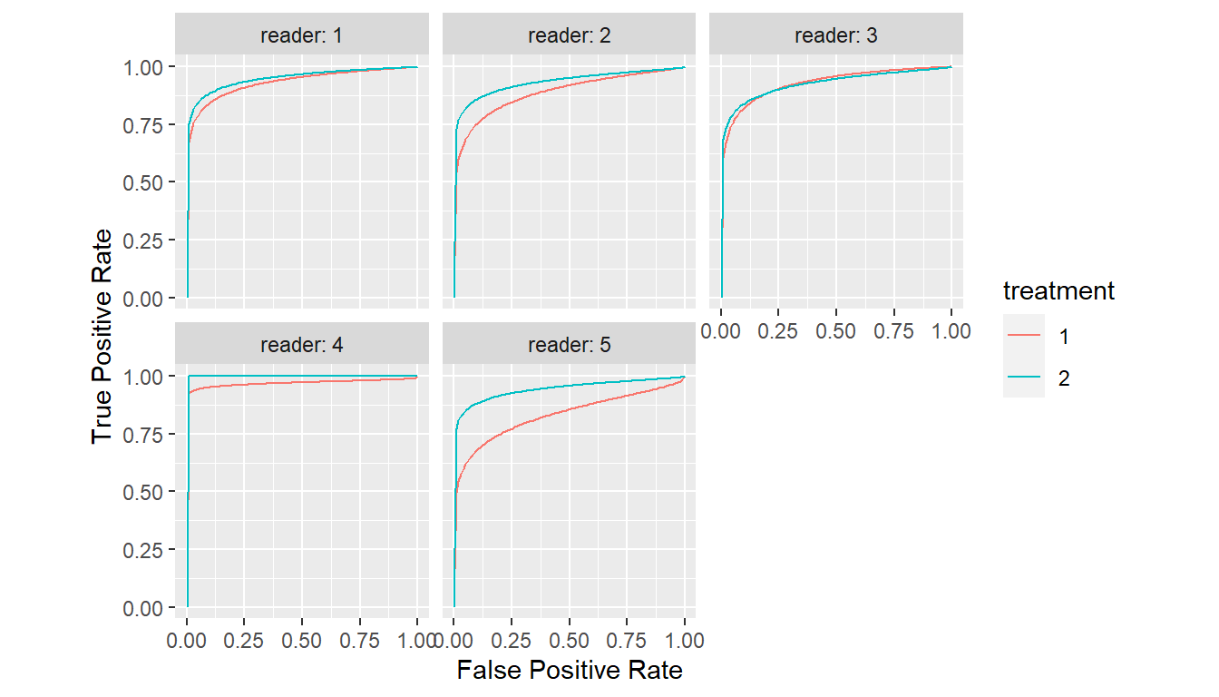
Show MRMC ROC Curve Parameters
print(parameters(est))
#> # A tibble: 10 × 3
#>    Group$reader $treatment      a     b
#>    <fct>        <fct>       <dbl> <dbl>
#>  1 1            1            1.70 0.537
#>  2 2            1            1.40 0.561
#>  3 3            1            1.74 0.635
#>  4 4            1            1.93 0.202
#>  5 5            1            1.06 0.464
#>  6 1            2            1.85 0.503
#>  7 2            2            1.66 0.447
#>  8 3            2            1.62 0.488
#>  9 4            2          Inf    1
#> 10 5            2            1.73 0.422
4.1.2 ROC Curve Expected Utility
As an alternative to AUC as a summary of ROC curves, Abbey et al. (2013) propose an expected utility metric defined as \[ \text{EU} = \max_\text{FPR}(\text{TPR}(\text{FPR}) - \beta \times \text{FPR}), \] where \(\text{TPR}(\text{FPR})\) are true positive rates on the ROC curve, and FPR are false positive rates ranging from 0 to 1.
ROC Curve Expected Utility Functions
binormal_eu(truth, rating, slope = 1)
binormalLR_eu(truth, rating, slope = 1)
empirical_eu(truth, rating, slope = 1)
trapezoidal_eu(truth, rating, slope = 1)Description
Returns expected utility of an ROC curve.
Arguments
truth: vector of true binary case statuses, with positive status taken to be the highest level.rating: numeric vector of case ratings.slope: numeric slope (\(\beta\)) at which to compute expected utility.
4.1.3 ROC Curve Sensitivity and Specificity
Functions are provided to extract sensitivity from an ROC curve for a given specificity and vice versa.
ROC Curve Sensitivity and Specificity Functions
binormal_sens(truth, rating, spec)
binormal_spec(truth, rating, sens)
binormalLR_sens(truth, rating, spec)
binormalLR_spec(truth, rating, sens)
empirical_sens(truth, rating, spec)
empirical_spec(truth, rating, sens)
trapezoidal_sens(truth, rating, spec)
trapezoidal_spec(truth, rating, sens)Description
Returns the sensitivity/specificity from an ROC curve at a specified specificity/sensitivity.
Arguments
truth: vector of true binary case statuses, with positive status taken to be the highest level.rating: numeric vector of case ratings.spec,sens: specificity/sensitivity on the ROC curve at which to return sensitivity/specificity.
4.1.4 Binary Metrics
Metrics for binary reader ratings are also available.
Sensitivity and Specificity Functions
binary_sens(truth, rating)
binary_spec(truth, rating)Description
Returns the sensitivity or specificity.
Arguments
truth: vector of true binary case statuses, with positive status taken to be the highest level.rating: factor or numeric vector of 0-1 binary ratings.
## Compare sensitivity for binary classification
VanDyke$binary_rating <- VanDyke$rating >= 3
est <- mrmc(
  binary_sens(truth, binary_rating), treatment, reader, case, data = VanDyke
)
Show MRMC Performance Metrics
print(est)
#> Call:
#> mrmc(response = binary_sens(truth, binary_rating), test = treatment,
#>     reader = reader, case = case, data = VanDyke)
#>
#> Positive truth status: 1
#>
#> Response metric data:
#>
#> # A tibble: 10 × 2
#>        N data$binary_sens $treatment $reader
#>    <dbl>            <dbl> <fct>      <fct>
#>  1    45            0.889 1          1
#>  2    45            0.778 1          2
#>  3    45            0.822 1          3
#>  4    45            0.933 1          4
#>  5    45            0.689 1          5
#>  6    45            0.978 2          1
#>  7    45            0.822 2          2
#>  8    45            0.911 2          3
#>  9    45            1     2          4
#> 10    45            0.889 2          5
#>
#> ANOVA Table:
#>
#>                  Df   Sum Sq   Mean Sq
#> treatment         1 0.023901 0.0239012
#> reader            4 0.049679 0.0124198
#> treatment:reader  4 0.007210 0.0018025
#>
#>
#> Obuchowski-Rockette error variance and covariance estimates:
#>
#>           Estimate Correlation
#> Error 0.0023681257          NA
#> Cov1  0.0009943883   0.4199052
#> Cov2  0.0010145903   0.4284360
#> Cov3  0.0006604938   0.2789100
Show MRMC Test Results
summary(est)
#> Multi-Reader Multi-Case Analysis of Variance
#> Data: VanDyke
#> Factor types: Random Readers and Random Cases
#> Covariance method: jackknife
#>
#> Experimental design: factorial
#>
#> Obuchowski-Rockette variance component and covariance estimates:
#>
#>                      Estimate Correlation
#> reader           0.0049747475          NA
#> treatment:reader 0.0007828283          NA
#> Error            0.0023681257          NA
#> Cov1             0.0009943883   0.4199052
#> Cov2             0.0010145903   0.4284360
#> Cov3             0.0006604938   0.2789100
#>
#>
#> ANOVA global test of equal treatment binary_sens:
#>        MS(T)     MS(T:R)       Cov2         Cov3 Denominator        F df1
#> 1 0.02390123 0.001802469 0.00101459 0.0006604938 0.003572952 6.689493   1
#>        df2    p-value
#> 1 15.71732 0.02008822
#>
#>
#> 95% CIs and tests for treatment binary_sens pairwise differences:
#>   Comparison    Estimate     StdErr       df   CI.Lower   CI.Upper         t
#> 1      1 - 2 -0.09777778 0.03780451 15.71732 -0.1780371 -0.0175185 -2.586405
#>      p-value
#> 1 0.02008822
#>
#>
#> 95% treatment binary_sens CIs (each analysis based only on data for the
#> specified treatment):
#>    Estimate       MS(R)        Cov2     StdErr        df  CI.Lower  CI.Upper
#> 1 0.8222222 0.009135802 0.001646465 0.05893747 14.456811 0.6961876 0.9482568
#> 2 0.9200000 0.005086420 0.000382716 0.03741657  7.575855 0.8328691 1.0000000
4.2 Covariance Estimation Methods
Special statistical methods are needed in MRMC analyses to estimate covariances between performance metrics from different readers and tests when cases are treated as a random sample and are rated by more than one reader or evaluated with more than one test. For this estimation, the package provides the DeLong method (DeLong, DeLong, and Clarke-Pearson 1988), jackknifing (Efron 1982), and an unbiased method (Gallas, Pennello, and Meyers 2007). The applicability of each depends on the study design as well as the performance metric being analyzed. DeLong is appropriate for a balanced factorial design and empirical ROC AUC, jackknifing for any design and metric, and unbiased for any design and empirical ROC AUC.
| Covariance Method | Study Design | Metric | Function |
|---|---|---|---|
| DeLong | Factorial | Empirical ROC AUC | DeLong() |
| Jackknife | Any | Any | jackknife() |
| Unbiased | Any | Empirical ROC AUC | unbiased() |
Jackknifing is the default covariance method for mrmc().
Others can be specified with its cov argument.
## DeLong method
est <- mrmc(
  empirical_auc(truth, rating), treatment, reader, case, data = VanDyke,
  cov = DeLong
)
Show MRMC Test Results
summary(est)
#> Multi-Reader Multi-Case Analysis of Variance
#> Data: VanDyke
#> Factor types: Random Readers and Random Cases
#> Covariance method: DeLong
#>
#> Experimental design: factorial
#>
#> Obuchowski-Rockette variance component and covariance estimates:
#>
#>                      Estimate Correlation
#> reader           0.0015364254          NA
#> treatment:reader 0.0002045840          NA
#> Error            0.0007921325          NA
#> Cov1             0.0003420090   0.4317573
#> Cov2             0.0003395265   0.4286234
#> Cov3             0.0002358497   0.2977402
#>
#>
#> ANOVA global test of equal treatment empirical_auc:
#>         MS(T)      MS(T:R)         Cov2         Cov3 Denominator        F df1
#> 1 0.004796171 0.0005510306 0.0003395265 0.0002358497 0.001069415 4.484854   1
#>        df2    p-value
#> 1 15.06611 0.05123303
#>
#>
#> 95% CIs and tests for treatment empirical_auc pairwise differences:
#>   Comparison    Estimate    StdErr       df      CI.Lower      CI.Upper
#> 1      1 - 2 -0.04380032 0.0206825 15.06611 -0.0878671960  0.0002665519
#>           t    p-value
#> 1 -2.117747 0.05123303
#>
#>
#> 95% treatment empirical_auc CIs (each analysis based only on data for the
#> specified treatment):
#>    Estimate       MS(R)         Cov2     StdErr       df  CI.Lower  CI.Upper
#> 1 0.8970370 0.003082629 0.0004775239 0.03307642 12.59597 0.8253461 0.9687280
#> 2 0.9408374 0.001304602 0.0002015292 0.02150464 12.56530 0.8942155 0.9874592
## Unbiased method
est <- mrmc(
  empirical_auc(truth, rating), treatment, reader, case, data = VanDyke,
  cov = unbiased
)
Show MRMC Test Results
summary(est)
#> Multi-Reader Multi-Case Analysis of Variance
#> Data: VanDyke
#> Factor types: Random Readers and Random Cases
#> Covariance method: unbiased
#>
#> Experimental design: factorial
#>
#> Obuchowski-Rockette variance component and covariance estimates:
#>
#>                      Estimate Correlation
#> reader           0.0015365290          NA
#> treatment:reader 0.0002077588          NA
#> Error            0.0007883925          NA
#> Cov1             0.0003416706   0.4333762
#> Cov2             0.0003390650   0.4300713
#> Cov3             0.0002356148   0.2988547
#>
#>
#> ANOVA global test of equal treatment empirical_auc:
#>         MS(T)      MS(T:R)        Cov2         Cov3 Denominator        F df1
#> 1 0.004796171 0.0005510306 0.000339065 0.0002356148 0.001068281 4.489614   1
#>        df2   p-value
#> 1 15.03418 0.0511618
#>
#>
#> 95% CIs and tests for treatment empirical_auc pairwise differences:
#>   Comparison    Estimate     StdErr       df      CI.Lower      CI.Upper
#> 1      1 - 2 -0.04380032 0.02067154 15.03418 -0.0878519409  0.0002512968
#>           t   p-value
#> 1 -2.118871 0.0511618
#>
#>
#> 95% treatment empirical_auc CIs (each analysis based only on data for the
#> specified treatment):
#>    Estimate       MS(R)         Cov2    StdErr       df  CI.Lower  CI.Upper
#> 1 0.8970370 0.003082629 0.0004771788 0.0330712 12.58802 0.8253526 0.9687214
#> 2 0.9408374 0.001304602 0.0002009512 0.0214912 12.53391 0.8942323 0.9874424
4.3 Fixed Factors
By default, readers and cases are treated as random effects by
mrmc(). Random effects are the appropriate designations
when inference is intended for the larger population from which study
readers and cases are considered to be a random sample. Either, but not
both, can be specified as fixed effects with the fixed()
function in applications where study readers or cases make up the entire
group to which inference is intended. When readers are designated as
fixed, mrmc() test results additionally include
reader-specific pairwise comparisons of the diagnostic tests as well as
mean estimates of the performance metric for each reader-test
combination.
## Fixed readers
est <- mrmc(
  empirical_auc(truth, rating), treatment, fixed(reader), case, data = VanDyke
)
Show MRMC Test Results
summary(est)
#> Multi-Reader Multi-Case Analysis of Variance
#> Data: VanDyke
#> Factor types: Fixed Readers and Random Cases
#> Covariance method: jackknife
#>
#> Experimental design: factorial
#>
#> Obuchowski-Rockette variance component and covariance estimates:
#>
#>                      Estimate Correlation
#> reader           0.0015349993          NA
#> treatment:reader 0.0002004025          NA
#> Error            0.0008022883          NA
#> Cov1             0.0003466137   0.4320314
#> Cov2             0.0003440748   0.4288668
#> Cov3             0.0002390284   0.2979333
#>
#>
#> ANOVA global test of equal treatment empirical_auc:
#>         MS(T)         Cov1         Cov2         Cov3  Denominator       X2 df
#> 1 0.004796171 0.0003466137 0.0003440748 0.0002390284 0.0008758604 5.475953  1
#>      p-value
#> 1 0.01927984
#>
#>
#> 95% CIs and tests for treatment empirical_auc pairwise differences:
#>   Comparison    Estimate     StdErr    CI.Lower    CI.Upper         z
#> 1      1 - 2 -0.04380032 0.01871748 -0.08048591 -0.00711473 -2.340075
#>      p-value
#> 1 0.01927984
#>
#>
#> 95% treatment empirical_auc CIs (each analysis based only on data for the
#> specified treatment):
#>    Estimate   Var(Error)         Cov2     StdErr  CI.Lower  CI.Upper
#> 1 0.8970370 0.0010141028 0.0004839618 0.02428971 0.8494301 0.9446440
#> 2 0.9408374 0.0005904738 0.0002041879 0.01677632 0.9079564 0.9737183
#>
#>
#> Reader-specific 95% CIs and tests for empirical_auc pairwise differences (each
#> analysis based only on data for the specified reader):
#>   Reader Comparison    Estimate     StdErr     CI.Lower     CI.Upper          z
#> 1      1      1 - 2 -0.02818035 0.02551213 -0.078183215  0.021822507 -1.1045864
#> 2      2      1 - 2 -0.04653784 0.02630183 -0.098088476  0.005012792 -1.7693768
#> 3      3      1 - 2 -0.01787440 0.03120965 -0.079044180  0.043295388 -0.5727202
#> 4      4      1 - 2 -0.02624799 0.01729129 -0.060138290  0.007642316 -1.5179891
#> 5      5      1 - 2 -0.10016103 0.04405746 -0.186512066 -0.013809995 -2.2734182
#>      p-value
#> 1 0.26933885
#> 2 0.07683102
#> 3 0.56683414
#> 4 0.12901715
#> 5 0.02300099
#>
#>
#> Single reader 95% CIs:
#>    empirical_auc treatment reader       StdErr  CI.Lower  CI.Upper
#> 1      0.9196457         1      1 0.0301255164 0.8606008 0.9786907
#> 2      0.8587762         1      2 0.0363753335 0.7874818 0.9300705
#> 3      0.9038647         1      3 0.0282594118 0.8484773 0.9592522
#> 4      0.9731079         1      4 0.0173388332 0.9391244 1.0000000
#> 5      0.8297907         1      5 0.0417201720 0.7480206 0.9115607
#> 6      0.9478261         2      1 0.0221416887 0.9044292 0.9912230
#> 7      0.9053140         2      2 0.0298151099 0.8468775 0.9637506
#> 8      0.9217391         2      3 0.0297673065 0.8633963 0.9800820
#> 9      0.9993559         2      4 0.0007213348 0.9979421 1.0000000
#> 10     0.9299517         2      5 0.0262023046 0.8785961 0.9813073
## Fixed cases
est <- mrmc(
  empirical_auc(truth, rating), treatment, reader, fixed(case), data = VanDyke
)
Show MRMC Test Results
summary(est)
#> Multi-Reader Multi-Case Analysis of Variance
#> Data: VanDyke
#> Factor types: Random Readers and Fixed Cases
#> Experimental design: factorial
#>
#> Obuchowski-Rockette variance component and covariance estimates:
#>
#> Not applicable because cases are fixed
#>
#>
#> ANOVA global test of equal treatment empirical_auc:
#>         MS(T)      MS(T:R)     F df1 df2    p-value
#> 1 0.004796171 0.0005510306 8.704   1   4 0.04195875
#>
#>
#> 95% CIs and tests for treatment empirical_auc pairwise differences:
#>   Comparison    Estimate df     StdErr    CI.Lower    CI.Upper         t
#> 1      1 - 2 -0.04380032  4 0.01484629 -0.08502022 -0.00258042 -2.950254
#>      p-value
#> 1 0.04195875
#>
#>
#> 95% treatment empirical_auc CIs (each analysis based only on data for the
#> specified treatment):
#>    Estimate       MS(R)     StdErr df  CI.Lower  CI.Upper
#> 1 0.8970370 0.003082629 0.02482994  4 0.8280981 0.9659760
#> 2 0.9408374 0.001304602 0.01615303  4 0.8959894 0.9856854
4.4 Study Designs
MRMCaov supports factorial, nested, and partially
paired study designs. In a factorial design, one set of cases is
evaluated by all readers and tests. This is the design employed by the
VanDyke study as indicated by its dataset case identifier
values which appear within each combination of the reader
and treatment identifiers. Designs in which a different set
of cases is evaluated by each reader or with each test can be specified
with unique codings of case identifiers within the corresponding nesting
factor. Example codings for these two nested designs are included in the
VanDyke dataset as case2 and
case3. The case2 identifiers differ from
reader to reader and thus represent a study design in which cases are
nested within readers. Likewise, the case3 identifiers
differ by test and are an example design of cases nested within tests.
Additionally, the package supports partially paired designs in which
ratings may not be available on all cases for some readers or tests;
e.g., as a result of missing values. Nested and partially paired designs
require specification of jackknife (default) or unbiased as the
covariance estimation method.
#> Case identifier codings for factorial and nested study designs
#>            Observation
#> Factor      1   2   3   4   5   6   7   8   9   10  11  12  13  14  15  16  17
#>   reader    1   1   2   2   3   3   4   4   5   5   1   1   2   2   3   3   4
#>   treatment 1   2   1   2   1   2   1   2   1   2   1   2   1   2   1   2   1
#>   case      1   1   1   1   1   1   1   1   1   1   2   2   2   2   2   2   2
#>   case2     1.1 1.1 2.1 2.1 3.1 3.1 4.1 4.1 5.1 5.1 1.2 1.2 2.2 2.2 3.2 3.2 4.2
#>   case3     1.1 2.1 1.1 2.1 1.1 2.1 1.1 2.1 1.1 2.1 1.2 2.2 1.2 2.2 1.2 2.2 1.2
#>            Observation
#> Factor      18  19  20  21  22  23  24  25  26  27  28  29  30
#>   reader    4   5   5   1   1   2   2   3   3   4   4   5   5
#>   treatment 2   1   2   1   2   1   2   1   2   1   2   1   2
#>   case      2   2   2   3   3   3   3   3   3   3   3   3   3
#>   case2     4.2 5.2 5.2 1.3 1.3 2.3 2.3 3.3 3.3 4.3 4.3 5.3 5.3
#>   case3     2.2 1.2 2.2 1.3 2.3 1.3 2.3 1.3 2.3 1.3 2.3 1.3 2.3
#> ... with 1110 more observations
## Cases nested within readers
est <- mrmc(
empirical_auc(truth, rating), treatment, reader, case2, data = VanDyke
)Show MRMC Test Results
summary(est)
#> Multi-Reader Multi-Case Analysis of Variance
#> Data: VanDyke
#> Factor types: Random Readers and Random Cases
#> Covariance method: jackknife
#>
#> Experimental design: cases nested within reader
#>
#> Obuchowski-Rockette variance component and covariance estimates:
#>
#>                      Estimate Correlation
#> reader           1.293517e-03          NA
#> treatment:reader 9.213005e-05          NA
#> Error            8.079682e-04          NA
#> Cov1             3.490676e-04   0.4320314
#> Cov2             0.000000e+00   0.0000000
#> Cov3             0.000000e+00   0.0000000
#>
#>
#> ANOVA global test of equal treatment empirical_auc:
#>         MS(T)      MS(T:R) Cov2 Cov3  Denominator     F df1 df2    p-value
#> 1 0.004796171 0.0005510306    0    0 0.0005510306 8.704   1   4 0.04195875
#>
#>
#> 95% CIs and tests for treatment empirical_auc pairwise differences:
#>   Comparison    Estimate     StdErr df    CI.Lower    CI.Upper         t
#> 1      1 - 2 -0.04380032 0.01484629  4 -0.08502022 -0.00258042 -2.950254
#>      p-value
#> 1 0.04195875
#>
#>
#> 95% treatment empirical_auc CIs (each analysis based only on data for the
#> specified treatment):
#>    Estimate       MS(R) Cov2     StdErr df  CI.Lower  CI.Upper
#> 1 0.8970370 0.003082629    0 0.02482994  4 0.8280981 0.9659760
#> 2 0.9408374 0.001304602    0 0.01615303  4 0.8959894 0.9856854
## Cases nested within tests
est <- mrmc(
  empirical_auc(truth, rating), treatment, reader, case3, data = VanDyke
)
Show MRMC Test Results
summary(est)
#> Multi-Reader Multi-Case Analysis of Variance
#> Data: VanDyke
#> Factor types: Random Readers and Random Cases
#> Covariance method: jackknife
#>
#> Experimental design: cases nested within treatment
#>
#> Obuchowski-Rockette variance component and covariance estimates:
#>
#>                      Estimate Correlation
#> reader           1.642585e-03          NA
#> treatment:reader 9.078969e-05          NA
#> Error            8.058382e-04          NA
#> Cov1             0.000000e+00   0.0000000
#> Cov2             3.455973e-04   0.4288668
#> Cov3             0.000000e+00   0.0000000
#>
#>
#> ANOVA global test of equal treatment empirical_auc:
#>         MS(T)      MS(T:R)         Cov2 Cov3 Denominator        F df1      df2
#> 1 0.004796171 0.0005510306 0.0003455973    0 0.002279017 2.104491   1 68.42325
#>     p-value
#> 1 0.1514363
#>
#>
#> 95% CIs and tests for treatment empirical_auc pairwise differences:
#>   Comparison    Estimate     StdErr       df    CI.Lower    CI.Upper         t
#> 1      1 - 2 -0.04380032 0.03019283 68.42325 -0.10404242  0.01644178 -1.450686
#>     p-value
#> 1 0.1514363
#>
#>
#> 95% treatment empirical_auc CIs (each analysis based only on data for the
#> specified treatment):
#>    Estimate       MS(R)         Cov2     StdErr       df  CI.Lower  CI.Upper
#> 1 0.8970370 0.003082629 0.0004861032 0.03320586 12.79430 0.8251827 0.9688914
#> 2 0.9408374 0.001304602 0.0002050913 0.02158730 12.75962 0.8941114 0.9875634
5 Single-Reader Multi-Case Analysis
A single-reader multi-case (SRMC) analysis involves a single readers
of multiple cases to compare reader performance metrics across two or
more diagnostic tests. An SRMC analysis can be performed with a call to
srmc().
SRMC Function
srmc(response, test, case, data, cov = jackknife)Description
Returns an
srmcclass object of data that can be used to estimate and compare reader performance metrics in a single-reader multi-case statistical analysis.Arguments
response: object defining true case statuses, corresponding reader ratings, and a reader performance metric to compute on them.test,case: variables containing the test and case identifiers for theresponseobservations.data: data frame containing the response and identifier variables.cov: functionjackknife,unbiased, orDeLongto estimate reader performance metric covariances.
The function is used similar to mrmc() but without the
reader argument. Below is an example SRMC analysis
performed with one of the readers from the VanDyke
dataset.
## Subset VanDyke dataset by reader 1
VanDyke1 <- subset(VanDyke, reader == "1")

## Compare ROC AUC treatment means for reader 1
est <- srmc(binormal_auc(truth, rating), treatment, case, data = VanDyke1)
Show SRMC Performance Metrics
print(est)
#> Call:
#> srmc(response = binormal_auc(truth, rating), test = treatment,
#>     case = case, data = VanDyke1)
#>
#> Positive truth status: 1
#>
#> Response metric data:
#>
#> # A tibble: 2 × 2
#>       N data$binormal_auc $treatment $reader
#>   <dbl>             <dbl> <fct>      <fct>
#> 1   114             0.933 1          1
#> 2   114             0.951 2          1
#>
#> ANOVA Table:
#>
#>                  Df     Sum Sq    Mean Sq
#> treatment         1 0.00010393 0.00010393
#> reader            0 0.00000000 0.00000000
#> treatment:reader  0 0.00000000 0.00000000
#>
#>
#> Obuchowski-Rockette error variance and covariance estimates:
#>
#>           Estimate Correlation
#> Error 0.0008371345          NA
#> Cov1  0.0004275594   0.5107416
#> Cov2  0.0000000000   0.0000000
#> Cov3  0.0000000000   0.0000000
Show SRMC ROC Curves
plot(est)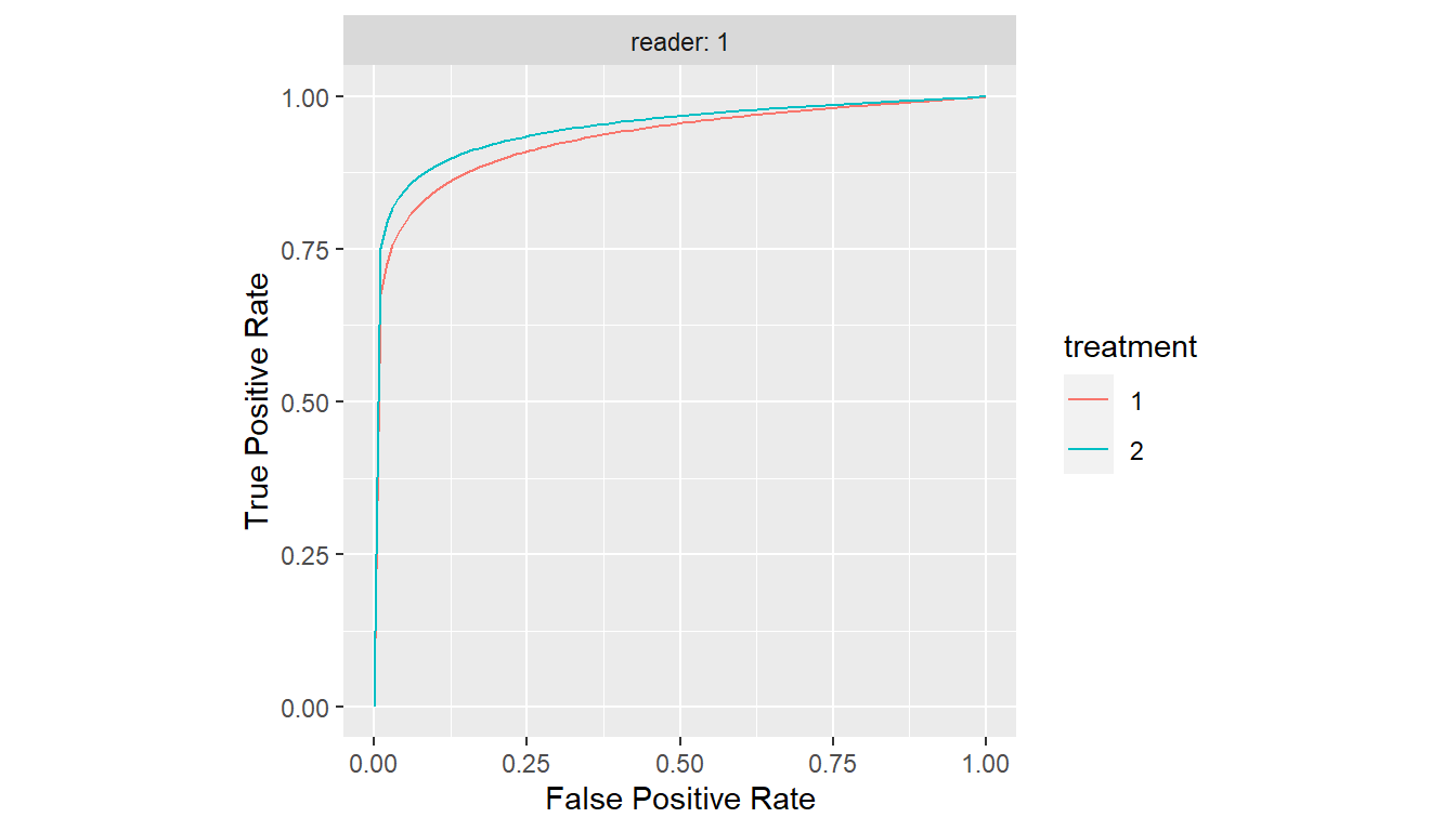
Show SRMC ROC Curve Parameters
print(parameters(est))
#> # A tibble: 2 × 3
#>   Group$reader $treatment     a     b
#>   <fct>        <fct>      <dbl> <dbl>
#> 1 1            1           1.70 0.537
#> 2 1            2           1.85 0.503
Show SRMC Test Results
summary(est)
#> Single-Reader Multi-Case Analysis of Variance
#> Data: VanDyke1
#> Factor types: Fixed Readers and Random Cases
#> Covariance method: jackknife
#>
#> Experimental design: cases nested within reader
#>
#> Obuchowski-Rockette variance component and covariance estimates:
#>
#>           Estimate Correlation
#> Error 0.0008371345          NA
#> Cov1  0.0004275594   0.5107416
#> Cov2  0.0000000000   0.0000000
#> Cov3  0.0000000000   0.0000000
#>
#>
#> 95% CIs and tests for treatment binormal_auc pairwise differences:
#>   Comparison    Estimate    StdErr    CI.Lower    CI.Upper         z  p-value
#> 1      1 - 2 -0.01765763 0.0286208 -0.07375337  0.03843810 -0.616951 0.537267
#>
#>
#> Single reader 95% CIs:
#>   binormal_auc treatment reader     StdErr  CI.Lower  CI.Upper
#> 1    0.9331609         1      1 0.03348342 0.8675346 0.9987872
#> 2    0.9508186         2      1 0.02351871 0.9047228 0.9969144
6 Single-Test Multi-Case Analysis
A single-test and single-reader multi-case (STMC) analysis involves a
single reader of multiple cases to estimate a reader performance metric
for one diagnostic test. An STMC analysis can be performed with a call
to stmc().
STMC Function
stmc(response, case, data, cov = jackknife)Description
Returns an
stmcclass object of data that can be used to estimate a reader performance metric in a single-test and single-reader multi-case statistical analysis.Arguments
response: object defining true case statuses, corresponding reader ratings, and a reader performance metric to compute on them.case: variable containing the case identifiers for theresponseobservations.data: data frame containing the response and identifier variables.cov: functionjackknife,unbiased, orDeLongto estimate reader performance metric covariances.
The function is used similar to mrmc() but without the
test and reader arguments. In the following
example, an STMC analysis is performed with one of the tests and readers
from the VanDyke dataset.
## Subset VanDyke dataset by treatment 1 and reader 1
VanDyke11 <- subset(VanDyke, treatment == "1" & reader == "1")

## Estimate ROC AUC for treatment 1 and reader 1
est <- stmc(binormal_auc(truth, rating), case, data = VanDyke11)
Show STMC ROC Curve
plot(est)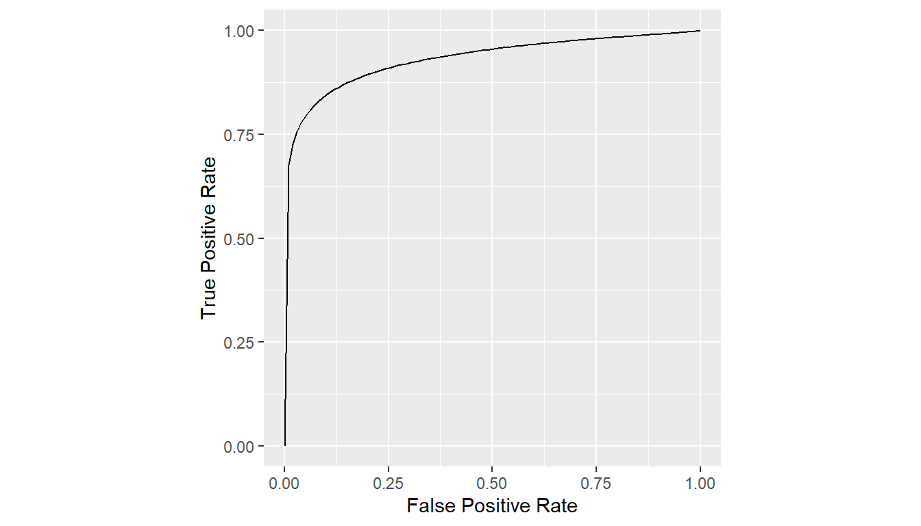
Show STMC ROC Curve Parameters
print(parameters(est))
#> # A tibble: 1 × 2
#>       a     b
#>   <dbl> <dbl>
#> 1  1.70 0.537
Show STMC ROC AUC Estimate
summary(est)
#> binormal_auc       StdErr     CI.Lower     CI.Upper
#>   0.93316094   0.03348342   0.86753465   0.99878723
7 ROC Curves
ROC curves can be estimated, summarized, and displayed apart from a
multi-case statistical analysis with the roc_curves()
function. Supported estimation methods include the empirical
distribution (default), binormal model, and binormal likelihood-ratio
model.
7.1 Curve Fitting
ROC Curves Function
roc_curves(truth, rating, groups = list(), method = "empirical")Description
Returns an
roc_curvesclass object of estimated ROC curves.Arguments
truth: vector of true binary case statuses, with positive status taken to be the highest level.rating: numeric vector of case ratings.groups: list or data frame of grouping variables of the same lengths astruthandrating.method: character string indicating the curve type as"binormal","binormalLR","empirical", or"trapezoidal".
A single curve can be estimated over all observations or multiple
curves estimated within the levels of one or more grouping variables.
Examples of both are given in the following sections using variables
from the VanDyke dataset referenced inside of calls to the
with() function. Alternatively, the variables may be
referenced with the $ operator; e.g.,
VanDyke$truth and VanDyke$rating. Resulting
curves from roc_curves() can be displayed with the
print() and plot() functions.
7.1.1 Single Curve
## Direct referencing of data frame columns
# curve <- roc_curves(VanDyke$truth, VanDyke$rating)

## Indirect referencing using the with function
curve <- with(VanDyke, {
  roc_curves(truth, rating)
})
plot(curve)
7.1.2 Multiple Curves
Multiple group-specific curves can be obtained from
roc_curves() by supplying a list or data frame of grouping
variables to the groups argument. Groups will be formed and
displayed in the order in which grouping variables are supplied. For
instance, a second grouping variable will be plotted within the first
one.
## Grouped by reader
curves <- with(VanDyke, {
  roc_curves(truth, rating,
             groups = list(Reader = reader, Treatment = treatment))
})
plot(curves)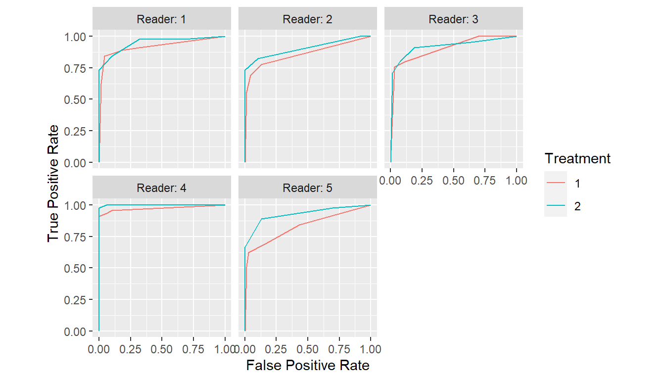
## Grouped by treatment
curves <- with(VanDyke, {
  roc_curves(truth, rating,
             groups = list(Treatment = treatment, Reader = reader))
})
plot(curves)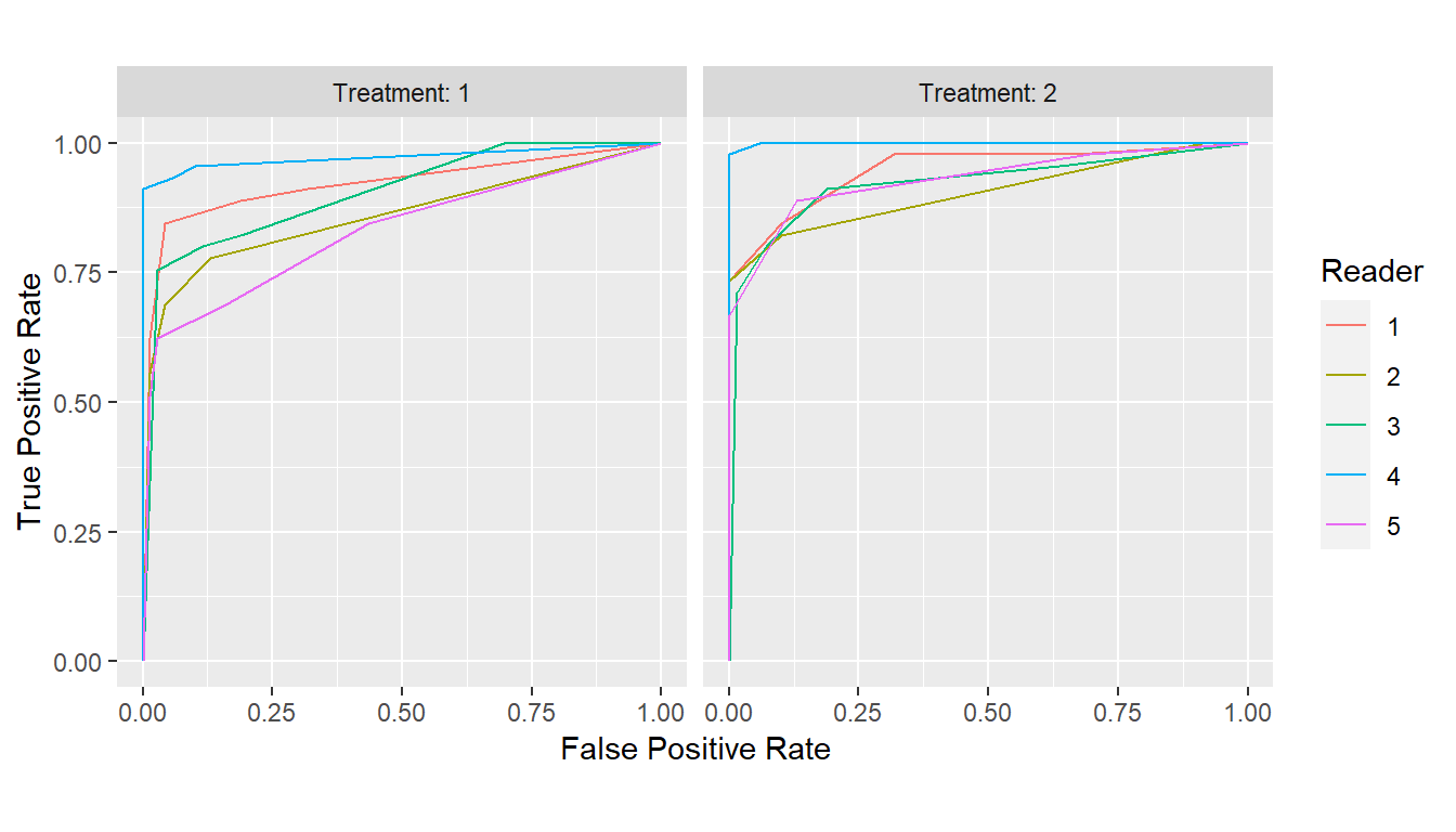
7.1.3 Parametric Curves
Estimated parameters for curves obtained with the binormal or
binormal likelihood-ratio models can be extracted as a data frame with
the parameters() function.
## Binormal curves
curves_binorm <- with(VanDyke, {
  roc_curves(truth, rating,
             groups = list(Treatment = treatment, Reader = reader),
             method = "binormal")
})
params_binorm <- parameters(curves_binorm)
print(params_binorm)
#> # A tibble: 10 × 3
#>    Group$Treatment $Reader      a     b
#>    <fct>           <fct>    <dbl> <dbl>
#>  1 1               1         1.70 0.537
#>  2 2               1         1.85 0.503
#>  3 1               2         1.40 0.561
#>  4 2               2         1.66 0.447
#>  5 1               3         1.74 0.635
#>  6 2               3         1.62 0.488
#>  7 1               4         1.93 0.202
#>  8 2               4       Inf    1
#>  9 1               5         1.06 0.464
#> 10 2               5         1.73 0.422
plot(curves_binorm)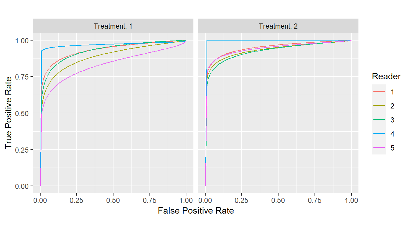
Estimates for different parameterizations of the binormal likelihood-ratio model are additionally returned and include those of the binormal model and the simplification of Pan and Metz (1997; Metz and Pan 1999) as well as those of the bi-chi-squared model (Hillis 2017).
## Binormal likelihood-ratio curves
curves_binormLR <- with(VanDyke, {
roc_curves(truth, rating,
groups = list(Treatment = treatment, Reader = reader),
method = "binormalLR")
})
params_binormLR <- parameters(curves_binormLR)
print(params_binormLR)
#> # A tibble: 10 × 4
#> Group$Treatment $Reader Metz$d_a $c bichisquared…¹ $theta binorma…²
#> <fct> <fct> <dbl> <dbl> <dbl> <dbl> <dbl>
#> 1 1 1 2.13 -0.298 3.42 1.71e+ 0 1.71e+0
#> 2 2 1 2.35 -0.321 3.79 1.70e+ 0 1.87e+0
#> 3 1 2 1.73 -0.281 3.17 1.32e+ 0 1.40e+0
#> 4 2 2 0.00700 -0.791 73.3 3.48e- 7 4.99e-3
#> 5 1 3 0.0140 -0.746 47.0 2.22e- 6 9.99e-3
#> 6 2 3 2.08 -0.330 3.94 1.23e+ 0 1.65e+0
#> 7 1 4 0.000417 -0.932 797. 1.09e-10 2.95e-4
#> 8 2 4 Inf 0 1 Inf Inf
#> 9 1 5 0.895 -0.508 9.37 5.94e- 2 6.66e-1
#> 10 2 5 2.02 -0.553 12.1 2.18e- 1 1.49e+0
#> # … with 1 more variable: binormal$b <dbl>, and abbreviated variable names
#> # ¹bichisquared$lambda, ²binormal$a
plot(curves_binormLR)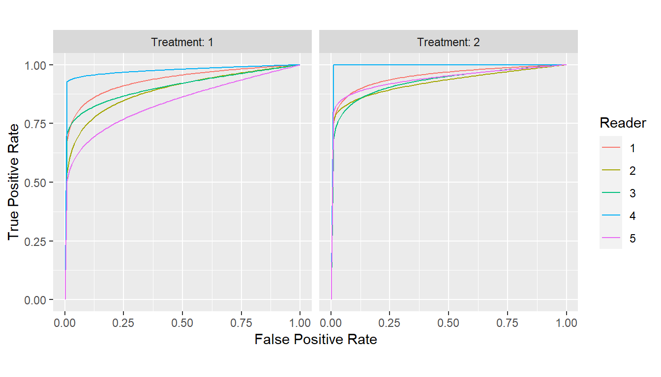
7.2 Curve Points
Points on an ROC curve estimated with roc_curves() can
be extracted with the points() function. True positive
rates (TPRs) and false positive rates (FPRs) on the estimated curve are
returned for a given set of sensitivity or specificity values or, in the
case of empirical curves, the original points. ROC curve points can be
displayed with print() and plot().
ROC Points Function
## Method for class 'roc_curves'
points(x, metric = "specificity", values = seq(0, 1, length = 101), ...)
## Method for class 'empirical_curves'
points(x, metric = "specificity", values = NULL, which = "curve", ...)Description
Returns an
roc_pointsclass object that is a data frame of false positive and true positive rates from an estimated ROC curve.Arguments
x: object fromroc_curves()for which to compute points on the curves.metric: character string specifying"specificity"or"sensitivity"as the reader performance metric to whichvaluescorrespond.values: numeric vector of values at which to compute ROC curve points, orNULLfor default empirical values as determined bywhich.which: character string indicating whether to use curve-specific observed values and 0 and 1 ("curve"), the combination of these values over all curves ("curves"), or only the observed curve-specific values ("observed").
## Extract points at given specificities
curve_spec_pts <- points(curves, metric = "spec", values = c(0.5, 0.7, 0.9))
print(curve_spec_pts)
#> # A tibble: 30 × 3
#>    Group$Treatment $Reader   FPR   TPR
#>  * <fct>           <fct>   <dbl> <dbl>
#>  1 1               1         0.1 0.862
#>  2 1               1         0.3 0.908
#>  3 1               1         0.5 0.935
#>  4 2               1         0.1 0.843
#>  5 2               1         0.3 0.966
#>  6 2               1         0.5 0.978
#>  7 1               2         0.1 0.747
#>  8 1               2         0.3 0.821
#>  9 1               2         0.5 0.872
#> 10 2               2         0.1 0.821
#> # … with 20 more rows
plot(curve_spec_pts, coord_fixed = FALSE)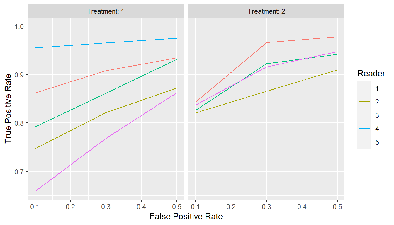
## Extract points at given sensitivities
curve_sens_pts <- points(curves, metric = "sens", values = c(0.5, 0.7, 0.9))
print(curve_sens_pts)
#> # A tibble: 30 × 3
#>    Group$Treatment $Reader    FPR   TPR
#>  * <fct>           <fct>    <dbl> <dbl>
#>  1 1               1       0.0116   0.5
#>  2 1               1       0.0246   0.7
#>  3 1               1       0.254    0.9
#>  4 2               1       0        0.5
#>  5 2               1       0        0.7
#>  6 2               1       0.337    0.9
#>  7 1               2       0.0130   0.5
#>  8 1               2       0.0543   0.7
#>  9 1               2       0.609    0.9
#> 10 2               2       0        0.5
#> # … with 20 more rows
plot(curve_sens_pts, coord_fixed = FALSE)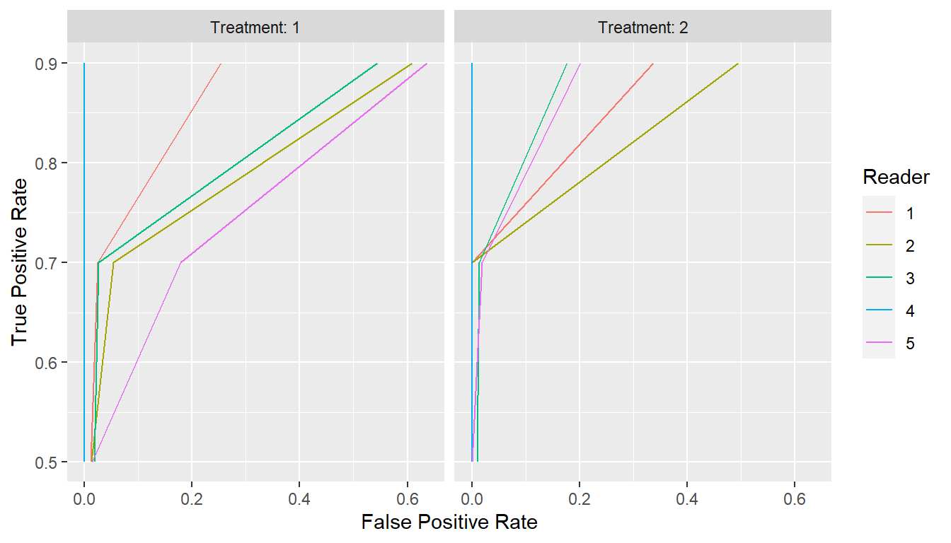
7.3 Mean Curves
A mean ROC curve from multiple group-specific curves returned by
roc_curves() can be computed with the means()
function. Curves can be averaged over sensitivities, specificities, or
binormal parameters (Chen and Samuelson
2014). Averaged curves can be displayed with print()
and plot().
ROC Means Function
## Method for class 'roc_curves'
mean(x, ...)
## Method for class 'binormal_curves'
mean(x, method = "points", ...)Description
Returns an
roc_pointsclass object.Arguments
x: object fromroc_curves()for which to average over the curves.method: character string indicating whether to average binormal curves over"points"or"parameters"....: optional arguments passed topoints(), including at whichmetric("sensitivity"or"specificity") values to average points on the ROC curves.
## Average sensitivities at given specificities (default)
curves_mean <- mean(curves)
print(curves_mean)
#> # A tibble: 20 × 2
#>       FPR   TPR
#>  *  <dbl> <dbl>
#>  1 0      0
#>  2 0      0.402
#>  3 0.0145 0.686
#>  4 0.0290 0.762
#>  5 0.0435 0.790
#>  6 0.0580 0.802
#>  7 0.0725 0.813
#>  8 0.101  0.835
#>  9 0.116  0.844
#> 10 0.130  0.852
#> 11 0.159  0.862
#> 12 0.188  0.872
#> 13 0.319  0.904
#> 14 0.362  0.912
#> 15 0.435  0.925
#> 16 0.638  0.956
#> 17 0.667  0.961
#> 18 0.696  0.966
#> 19 0.913  0.992
#> 20 1      1
plot(curves_mean)
## Average specificities at given sensitivities
curves_mean <- mean(curves, metric = "sens")
print(curves_mean)
#> # A tibble: 23 × 2
#>        FPR   TPR
#>  *   <dbl> <dbl>
#>  1 0       0
#>  2 0.00698 0.511
#>  3 0.00804 0.556
#>  4 0.00899 0.578
#>  5 0.00995 0.6
#>  6 0.0109  0.622
#>  7 0.0214  0.667
#>  8 0.0280  0.689
#>  9 0.0358  0.711
#> 10 0.0450  0.733
#> # … with 13 more rows
plot(curves_mean)
8 Reader Performance Metrics
The reader performance metrics described previously for use with
mrmc() and related functions to analyze multi and
single-reader multi-case studies can be applied to truth and rating
vectors as stand-alone functions. This enables estimation of performance
metrics for other applications, such as predictive modeling, that may be
of interest.
8.1 ROC Curve Metrics
AUC, partial AUC, sensitivity, and specificity are estimated below
with an empirical ROC curve. Estimates with binormal and binormal
likelihood-ratio curves can be obtained by replacing
empirical in the function names with binormal
and binormalLR, respectively.
## Total area under the empirical ROC curve
empirical_auc(VanDyke$truth, VanDyke$rating)
#> [1] 0.9229791

## Partial area for specificity from 0.7 to 1.0
empirical_auc(VanDyke$truth, VanDyke$rating, partial = "spec", min = 0.70, max = 1.0)
#> [1] 0.2499923

## Partial area for sensitivity from 0.7 to 1.0
empirical_auc(VanDyke$truth, VanDyke$rating, partial = "sens", min = 0.70, max = 1.0)
#> [1] 0.2262129

## Sensitivity for given specificity
empirical_sens(VanDyke$truth, VanDyke$rating, spec = 0.8)
#> [1] 0.8812346

## Sensitivity for given specificity
empirical_spec(VanDyke$truth, VanDyke$rating, sens = 0.8)
#> [1] 0.94434
8.2 Binary Metrics
Sensitivity and specificity for binary ratings are available with the
binary_sens() and binary_spec() functions as
demonstrated in the next example based on a binary rating created from
the numeric one in the VanDyke dataset.
## Create binary classification
VanDyke$binary_rating <- VanDyke$rating >= 3

## Sensitivity
binary_sens(VanDyke$truth, VanDyke$binary_rating)
#> [1] 0.8711111

## Specificity
binary_spec(VanDyke$truth, VanDyke$binary_rating)
#> [1] 0.8478261